Lecture 7 - Probability distribution
76
One of the most important things to know about a variable
is its distribution. Knowledge of the probability
distribution of the variables provides the clinicians and
researchers with a powerful tool for summarization and
describing a set of data and for reaching conclusion about
population on the basis of a sample drawn from that
population. We have several types of distribution in
statistics, but the "normal distribution" is the most
important one.
A probability distribution defines the relationship between
the outcomes and their likelihood of occurrence.
We have
several types of distribution in statistics:
I. For discrete variables we have
a) Binomial Distribution: dichotomous outcomes (A-B,
heads-tails, yes-no, on-off, is-is not, right-wrong, etc.)
b) Poisson Distribution Useful for studying rare random
events.
II. But the “Normal distribution" "Gaussian
distribution", for continues variables is the most
important one. This is because:
Many human variables naturally have a “bell shaped”
distribution.
The distributions are tied to probabilities, and it is the
probability which will be of interest to us
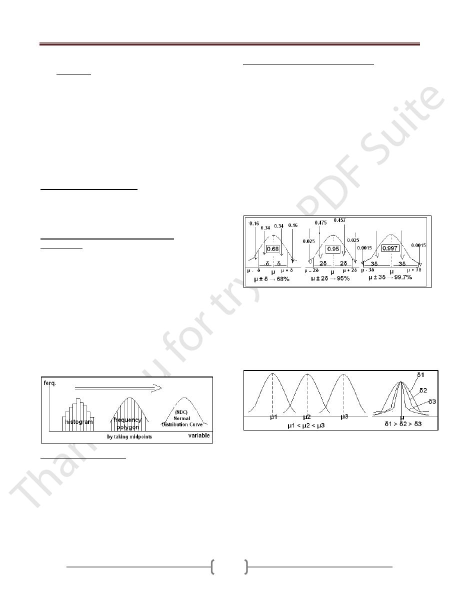
If we have a group of continuous variables with certain
class interval, we can represent them by histogram and
frequency polygon. But suppose we have a group of
variables which is huge and the class interval is very
small so the frequency polygon will take a shape of very
smooth curve & that curve is called "normal distribution
curve"
The normal distribution
"Gaussian distribution",
"Bell Shaped distribution" is the most important
distribution in the statistics, the parameters of this
distributions are:
1) The mean (µ) → Measure of location.
2) The standard deviation (∂) →Measure of dispersion.
Characteristic of the normal distribution
1) Used for the continuous variables, between
2) Symmetrical about its mean (µ), ((either side of mean is a
mirror image of other side.
3) Mean, median, and mode are equal.
4) The total area under the curve is equal to one, 50% on the
left &50% on the right of a perpendicular erected at the
mean.
5) The normal distribution is completely determined by the
parameters (µ) & (∂). Different values of µ shift the graph
along the X-axis, while different values of ∂ shift the
graph along the Y-axis (determine the degree of flatness
or peakness of the graph).
6) µ ± 1∂ → 68% of the area.
µ ± 2∂ → 95% of the area.
µ ± 3∂ → 99.7% of the area.
Different values of μ and δ shift the graph of distribution
along X & Y axes. If we change μ while keeping δ
constant, the curve will shift to the right on increasing μ
& to the left on decreasing μ. On changing δ and keeping
μ constant; the curve will become more flat on increasing
δ and narrower on decreasing δ without any shifting the
curve to any side. μ1 < μ2 < μ3
Since we know the shape of the curve, we can (using
calculus) calculate the area under the curve
The percentage of that area can be used to determine the
probability that a given value could be pulled from a
given distribution.
Each normal distribution with its own values of m and s
(unit) would need its own calculation of the area under
various points on the curve
Lecture 7 - Probability distribution
77
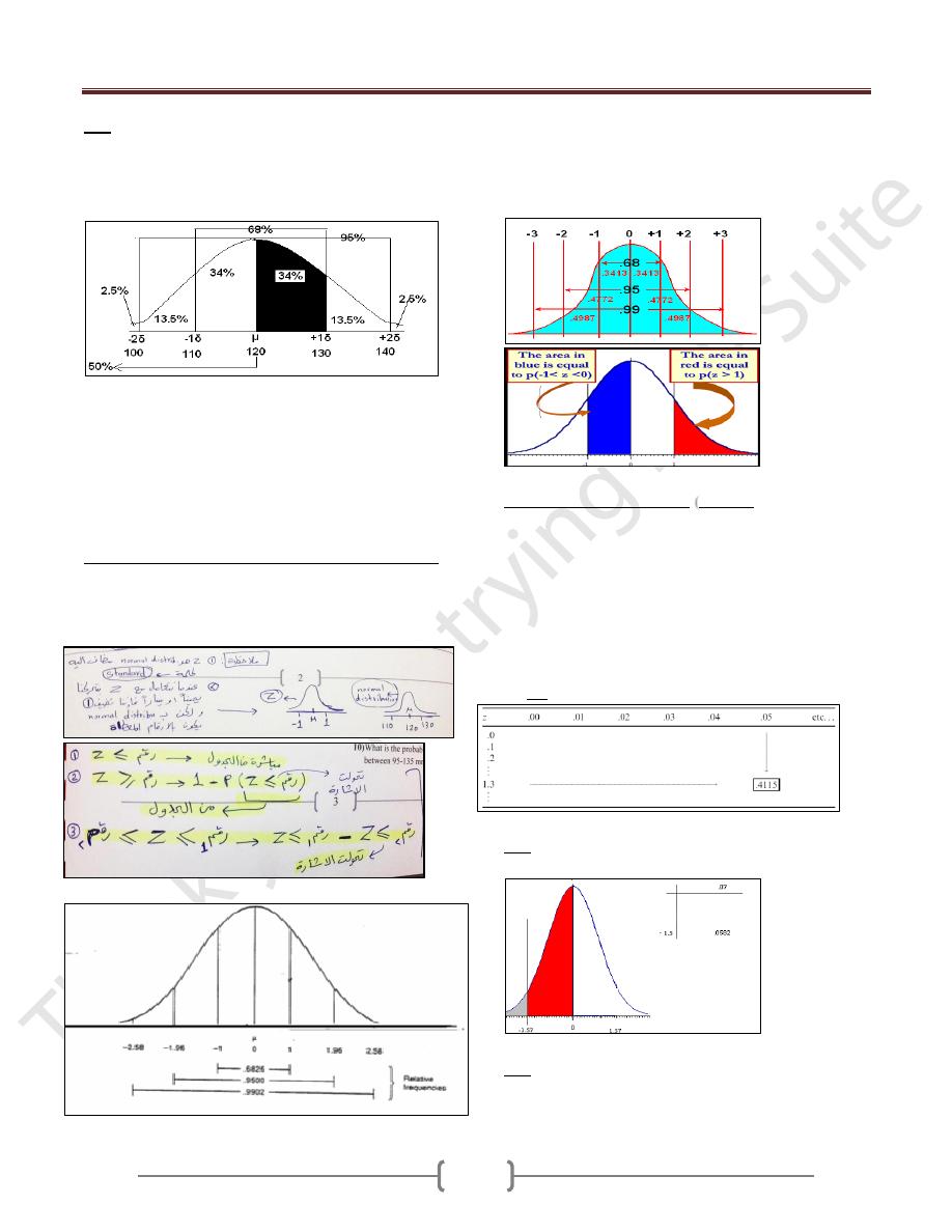
If population mean of systolic blood pressure is 120
x:
E
mmHg with population standard deviation of 10 mmHg.
What is the probability of getting a patient with systolic
BP a) between 120 and 130 mmHg, b) < 120mmHg, c) <
100 mmHg d) between 120 and 125 mmHg?
Answers:
a) From 120 to 130 we move one δ, so the probability is
34% (0.34) (i.e. half of 68%).
b) Probability of less than 120 mmHg is 50%.
c) Probability of less than 100 mmHg is 2.5%.
d) Probability of SBP between 120 and 125 mmHg; we
must follow Z scale.
The standard normal distribution
“Z-distribution".
It's the normal distribution curve which has a mean of
zero and a standard deviation of one (µ=0, & ∂ =1). →
Z = x - µ/ ∂
If we know the population means and population standard
deviation, for any value of X we can compute a z-score by
subtracting the population mean and dividing the result by
the population standard deviation
Properties of Z Distribution
Z-score)
(
90% of the values of a normal variable lie within
1.65
sample standard deviations from the sample mean
95% of the values of a normal variable lie within
1.96
sample standard deviations from the sample mean
99% of the values of a normal variable lie within
2.58
sample standard deviations from the sample mean
How to Read Z Table ((Must understand Z table, area to
the left))
Ex: Find p(Z<-1.57)
From Z table=0.0582
EX: From Z table: Find P (z ≥ 1.58)
P(z < 1.58) = 0.9429
P(z > 1.58) = 1 - 0.9429 = 0.0571
Lecture 7 - Probability distribution
78
Ex: From Z table find: Pr(-1 < z < 1) = 0:6826
Ex: Find p(0<Z<1.23)
Ex:
Calculate p(-1.2<Z<0.78)
p(-1.2<Z<0.78)= 0.7823-0.1151=0.6672
Ex:
Calculate p(-1.2<Z<0.78)
p(-1.2<Z<0.78)= 0.7823-0.1151=0.6672
Ex: What is the probability of having a patient with B.P
between 110-130 mm Hg? µ=120, ∂ =10. ((Suppose the
B.P is normally distributed)).
Z = x - µ/ ∂
= 110-120/10 =-1
= 130-120/10 = +1
P (110≤ x ≤ 130) → P(-1≤ Z ≤+ 1). &From the Z-table,
P=0.68.
Ex2: What is the probability of having a patient with B.P
above 140mm Hg?
Z = x - µ/ ∂
= 140-120/10 = +2
P(x ≥ 140) → P ( Z ≥ +2). &From the Z-table,
P=0.023.
Ex: If the total cholesterol values for a certain target
population are approximately normally distributed with a
mean of 200 (mg/100 mL) and a standard deviation of 20
(mg/100 mL), what is the probability that a person picked
at random from this population will have a cholesterol
value greater than 240 (mg/100 mL)?
Z = x - µ/ ∂ = 240-200/ 20 = 2
P (x >240) → P(Z > 2). = 0:0228 or 2.28%
Ex: in certain population the mean of SBP (µ=120), and ∂
=10mmHg. What is the probability of having a patient
with B.P between 110-130 mm Hg?
1) What is the probability of having a patient with B.P
between 105-125 mm Hg?
2) What is the probability of having a patient with B.P ≤
100 Hg?
3) What is the probability of having a patient with B.P ≥
135 mm Hg?
4) What is the probability of having a patient with B.P
between 120-140 mm Hg?
5) What is the probability of having a patient with B.P
between 100-140 mm Hg?
6) What is the probability of having a patient with B.P
between 90-150 mm Hg?
7) What is the probability of having a patient with B.P
between ≥ 150 mm Hg?
8) What is the probability of having a patient with B.P
between ≤150 mm Hg?
9) What is the probability of having a patient with B.P
between 140-150 mm Hg?

Lecture 7 - Probability distribution
79
10) What is the probability of having a patient with B.P
between 95-135 mm Hg?
EX: IQ’s are normally distributed with mean 100 and
standard deviation 15. Find the probability that a
randomly selected person has an IQ
1) between 100 and 115
2) More than 135.
3) Less than 70.
EX: A survey was done to measure the haemoglobin
(Hb) levels among a group of pregnant women attending
an ante-natal clinic. 10000 women were screened and the
mean Hb was found to be 10.5 gm%.The standard
deviation was 0.5. Compute:
1) Number of women having Hb level between 10 and 11
gm%
2) Number of women having Hb level between 9.5 and
11.5 gm%
3) Number of women having Hb level above 10.5 gm%.
4) Number of women having Hb level below 9 gm%.
5) Number of women having Hb level between 11 gm%
and 11.5 gm%.
6) Number of women having Hb level below 9 gm% and
above 12 gm%.
7) What is the probability of selecting a pregnant woman
with Hb levels below 10 gm%?