51
Lecture 7 - Regression
Regression allows you to predict variables based on another variable. Let’s begin with the
example used in the text in which mental health symptoms are predicted from stress.
Open symptoms and stress.sav.
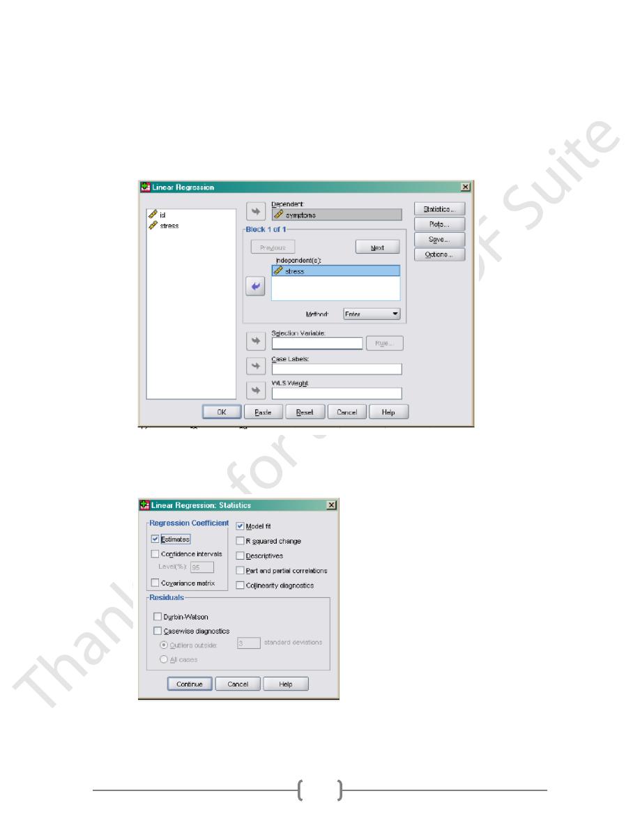
Select Analyze/Regression/Linear.
Figure 1
Select symptoms as the Dependent variable and stress as the Independent variable.
Then, click on Statistics to explore our options. The following dialog box will appear.
Figure 2
As you can see there are many options. Estimates and Model Fit are selected by default.
Leave them that way. Then select Descriptives and Part and partial correlations. SPSS
52
will then calculate the mean and standard deviation for each variable in the equation and the
correlation between the two variables. Then, click Continue.
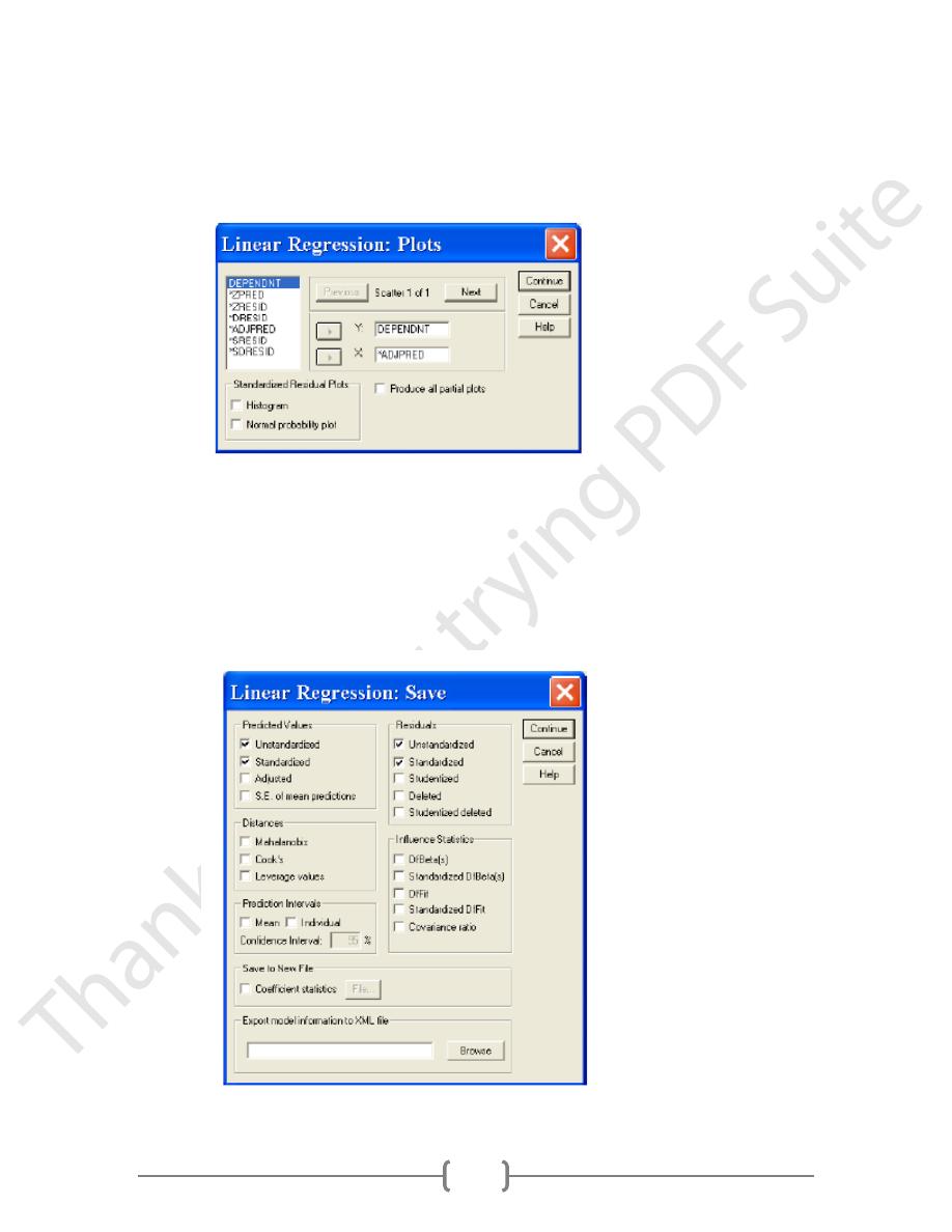
At the main dialog box, click on Plots so we can see our options.
Figure 3
It looks like we can create scatterplots here. Click Help to see what the abbreviations
represent. I’d like to plot the Dependent variable against the predicted values to see how
close they are. Select Dependnt for Y and Adjpred for X. Adjpred is the adjusted prediction.
Used Help/Topics/Index to find out what this means for yourself. Then, click Continue.
Figure 4
53
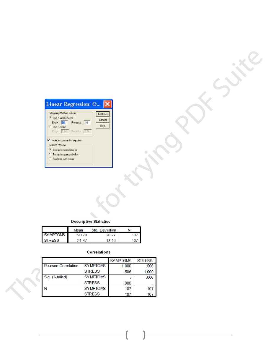
In the main dialog box, click Save, and the dialog box to the left will appear. For
Predicted Values, select Unstandardized and Standardized. For Residuals, also select
Unstandardized and Standardized. Now, SPSS will save the predicted values of symptoms
based on the regression equation and the residual or difference between the predicted values
and actual values of symptoms in the data file. This is a nice feature. Remember, the
standardized values are based on z score transformations of the data whereas the
unstandardized values are based on the raw data. Click Continue.
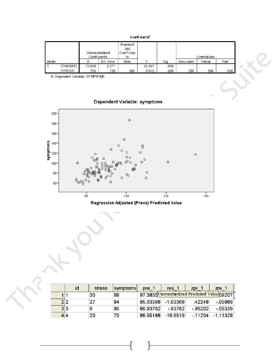
Finally, click on Options.
Including a constant in the equation is selected by default. This simply means that you
want both a slope and an intercept (the constant). That’s good. We will always leave this
checked. Excluding cases listwise is also fine. We do not have any missing cases in this
example.
54
Take a moment to identify all of the key pieces of information. Find the regression
coefficients used to calculate the regression equation. One difference is that the text did not
include the scatterplot. What do you think of the scatterplot? Does it help you see that
predicting symptoms based on stress is a pretty good estimate
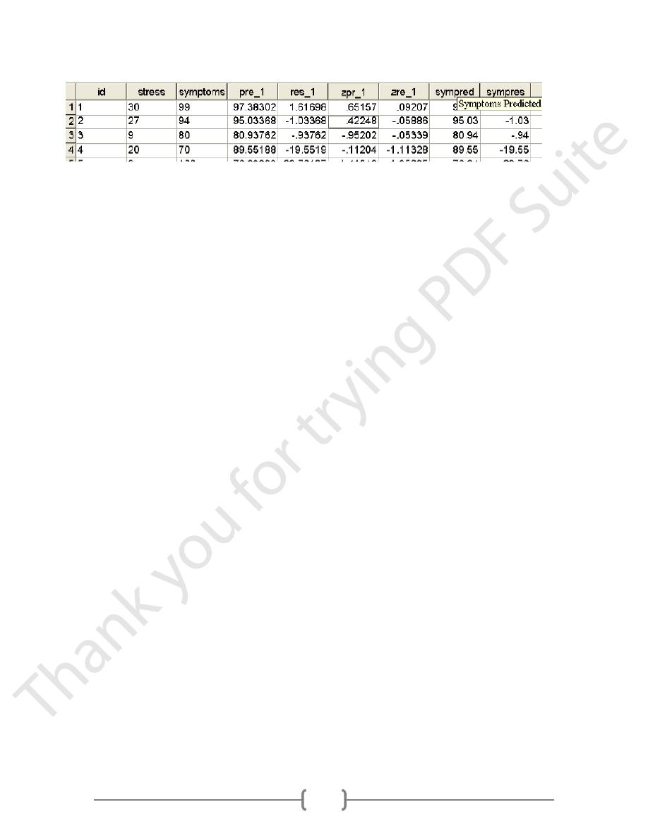
Now, click Window/Symptoms and stress.sav and look at the new data (residuals and
predicted values) in your file. A small sample is below. Note how they are named and
labeled.
55
Let’s use what we know about the regression equation to check the accuracy of the scores
created by SPSS. We will focus on the unstandardized predicted and residual values. This is
also a great opportunity to learn how to use the Transform menus to perform calculations
based on existing data.
We know from the regression equation that:
Symptoms Predicted or = 73.890 + .783* Stress. Yˆ
We also know that the residual can be computed as follows:
Residual = Y-or Symptoms – Symptoms Predicted Values. Yˆ
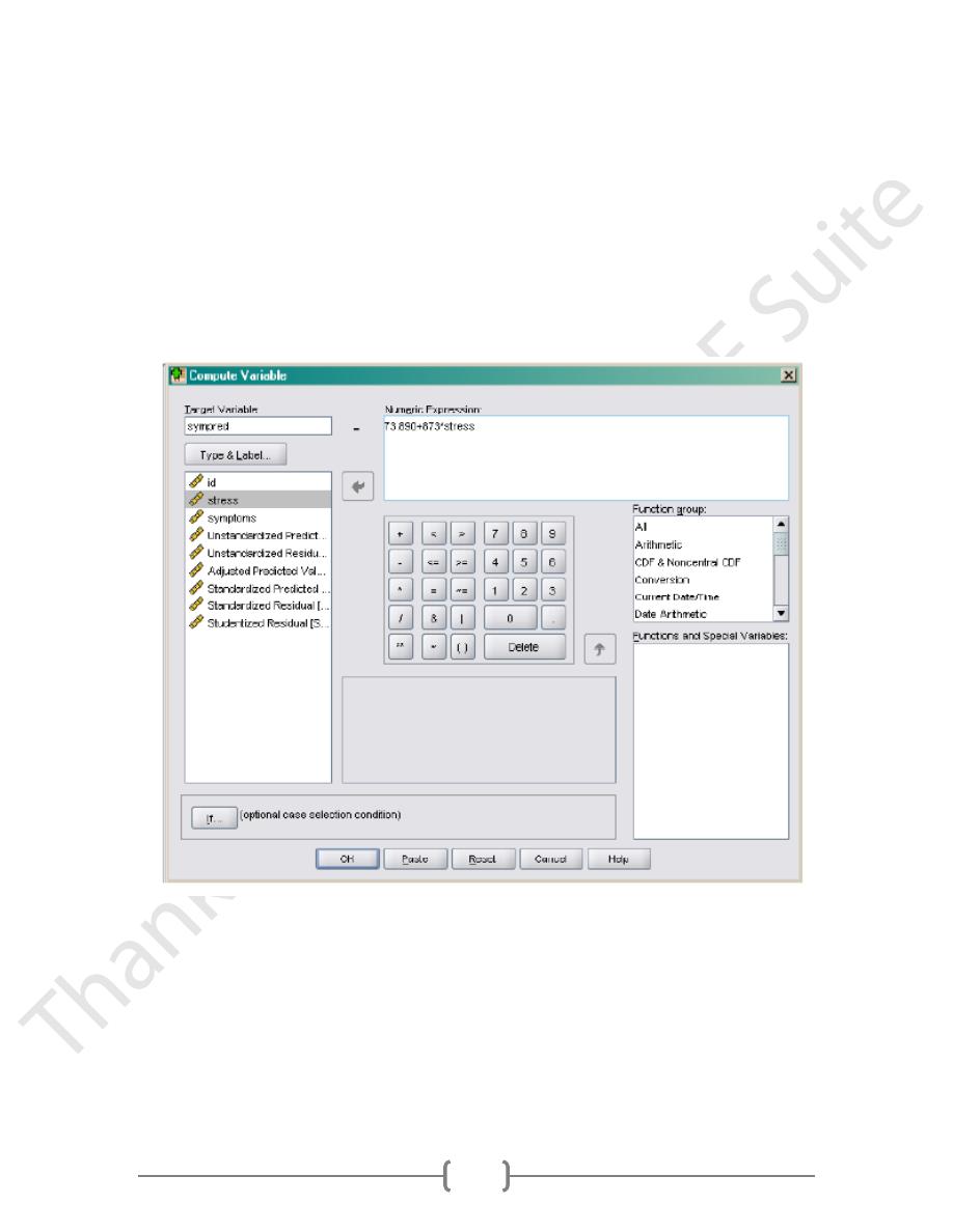
We’ll use SPSS to calculate these values and then compare them to the values computed by
SPSS.
In the Data Editor window, select Transform/Compute.
Check the Data Editor to see if your new variable is there, and compare it to pre_1. Are
they the same? The only difference I see is that our variable is only expressed to 2 decimal
places. But, the values agree.
Follow similar steps to calculate the residual. Click on Transform/Compute. Name your
Target Variable sympres and Label it symptoms residual. Put the formula symptoms-
sympred in the Numeric Expression box by double clicking the two pre-existing variables
and typing a minus sign between them. Then, click Ok.
Compare these values to res_1. Again they agree. A portion of the new data file is below.
56
Now that you are confident that the predicted and residual values computed by SPSS are
exactly what you intended, you won’t ever need to calculate them yourself again. You can
simply rely on the values computed by SPSS through the Save command.
