119
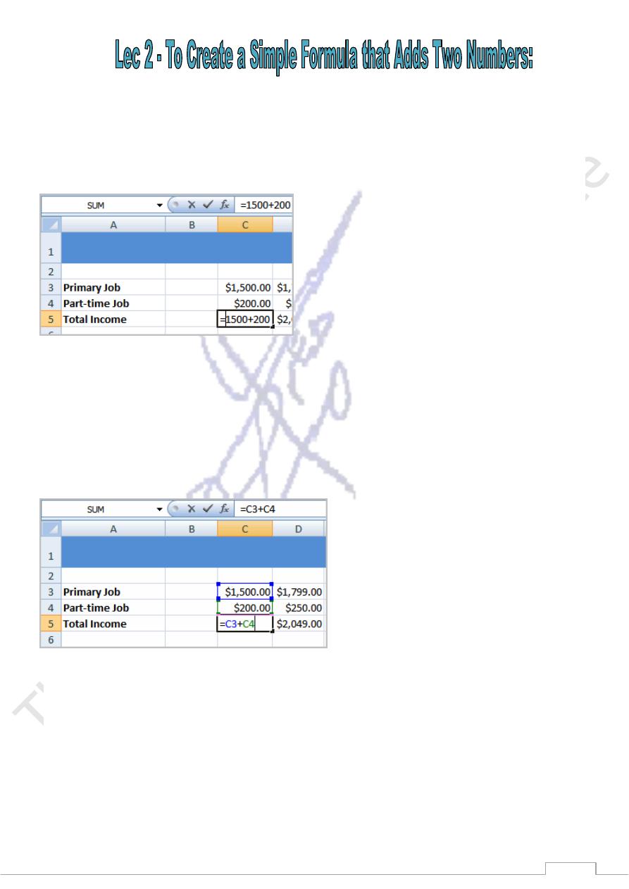
Click the cell where the formula will be defined (C5, for example).
Type the equal sign (=) to let Excel know a formula is being defined.
Type the first number to be added (e.g., 1500)
Type the addition sign (+) to let Excel know that an add operation is to be performed.
Type the second number to be added (e.g., 200)
Press Enter or click the Enter button on the Formula bar to complete the formula.
To Create a Simple Formula that Adds the Contents of Two Cells:
Click the cell where the answer will appear (C5, for example).
Type the equal sign (=) to let Excel know a formula is being defined.
Type the cell number that contains the first number to be added (C3, for example).
Type the addition sign (+) to let Excel know that an add operation is to be performed.
Type the cell address that contains the second number to be added (C4, for example).
Press Enter or click the Enter button on the Formula bar to complete the formula.
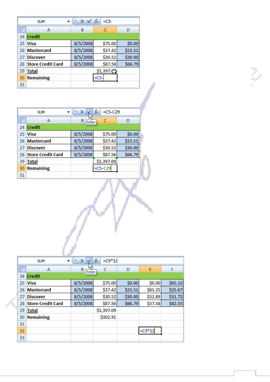
To Create a Simple Formula using the Point and Click Method:
Click the cell where the answer will appear (C30, for example).
Type the equal sign (=) to let Excel know a formula is being defined.
Click on the first cell to be included in the formula (C5, for example).
Type the subtraction sign (-) to let Excel know that a subtraction operation is to be performed.
Click on the next cell in the formula (C29, for example).
111
Press Enter or click the Enter button on the Formula bar to complete the formula.
To Create a Simple Formula that Multiplies the Contents of Two Cells:
Select the cell where the answer will appear (E32, for example).
Type the equal sign (=) to let Excel know a formula is being defined.
Click on the first cell to be included in the formula (C9, for example) or type a number.
Type the multiplication symbol (*) by pressing the Shift key and then the number 8 key. The
operator displays in the cell and Formula bar.
Click on the next cell in the formula or type a number (12, for example).
Press Enter or click the Enter button on the Formula bar to complete the formula.
111
To Create a Simple Formula that Divides One Cell by Another:
Click the cell where the answer will appear.
Type the equal sign (=) to let Excel know a formula is being defined.
Click on the first cell to be included in the formula.
Type a division symbol. The operator displays in the cell and Formula bar.
Click on the next cell in the formula.
Enter or click the Enter button on the Formula bar to complete the formula.
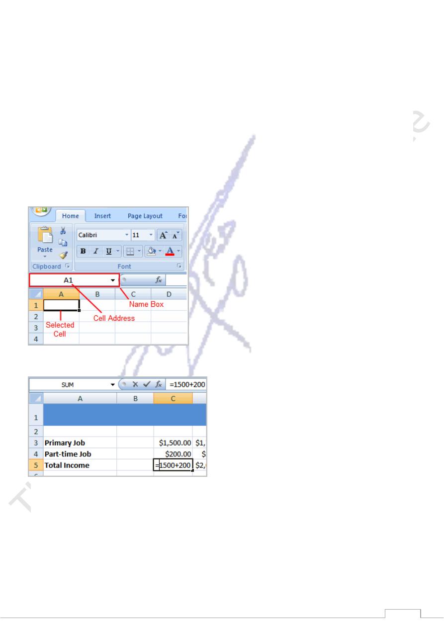
Using Cell References
As you can see, there are many ways to create a simple formula in Excel. Most likely you will choose one of
the methods that enters the cell address into the formula, rather than an actual number. The cell address is
basically the name of the cell and can be found in the Name Box.
The following example uses actual numbers in the formula in C5.
When a cell address is used as part of a formula, this is called a cell reference. It is called a cell reference
because instead of entering specific numbers into a formula, the cell address refers to a specific cell. The
following example uses cell references in the formula in C30.
112
Complex Formulas Defined
Simple formulas have one mathematical operation. Complex formulas involve more than one
mathematical operation.
Simple Formula: =2+2
Complex Formula: =2+2*8
To calculate complex formulas correctly, you must perform certain operations before others. This is defined
in the order of operations.
The Order of Operations
The order of mathematical operations is very important. If you enter a formula that contains several
operations, Excel knows to work those operations in a specific order. The order of operations is:
1. Operations enclosed in parenthesis
2. Exponential calculations (to the power of)
3. Multiplication and division, whichever comes first
4. Addition and subtraction, whichever comes first
A mnemonic that can help you remember this is Please Excuse My Dear Aunt Sally (P.E.M.D.A.S).
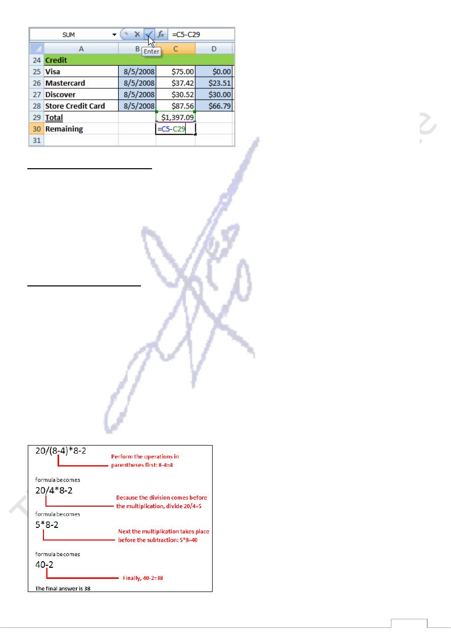
Example 1
Using this order, let us see how the formula 20/(8-4)*8-2 is calculated in the following breakdown:

113
Example 2
3+3*2=?
Is the answer 12 or 9? Well, if you calculated in the order in which the numbers appear, 3+3*2, you'd get the
wrong answer, 12. You must follow the order of operations to get the correct answer.
To Calculate the Correct Answer:
1. Calculate 3*2 first because multiplication comes before addition in the order of operations. The
answer is 6.
2. Add the answer obtained in step #1, which is 6, to the number 3 that opened the equation. In other
words, add 3 + 6.
3. The answer is 9.
Complex Formulas (continued)
Before moving on, let's explore some more formulas to make sure you understand the order of operations by
which Excel calculates the answer.
4*2/4
Multiply 4*2 before performing the
division operation because the
multiplication sign comes before the
division sign. The answer is 2.
4/2*4
Divide 4 by 2 before performing the
multiplication operation because the
division sign comes before the
multiplication sign. The answer is 8.
4/(2*4)
Perform the operation in parentheses
(2*4) first and divide 4 by this result. The
answer is 0.5.
4-2*4
Multiply 2*4 before performing the
subtraction operation because the
multiplication sign is of a higher order
than the subtraction sign. The answer is -
4.
Creating Complex Formulas
Excel automatically follows a standard order of operations in a complex formula. If you want a certain
portion of the formula to be calculated first, put it in parentheses.
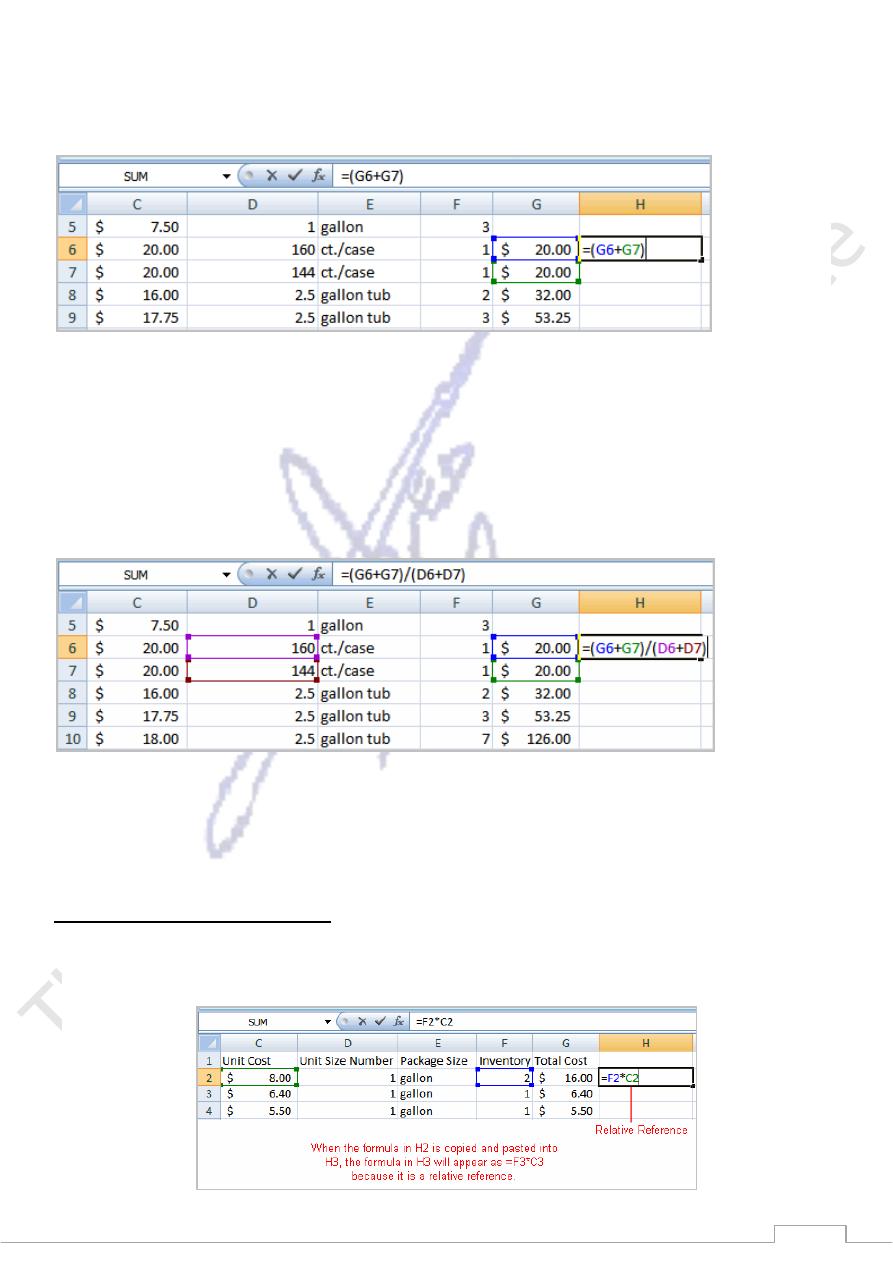
Example of How to Write a Complex Formula:
Click the cell where you want the formula result to appear. In this example, H6.
Type the equal sign (=) to let Excel know a formula is being defined.
Type an open parenthesis, or (
114
Click on the first cell to be included in the formula (G6, for example).
Type the addition sign (+) to let Excel know that an add operation is to be performed.
Click on the second cell in the formula (G7, for example)
Type a close parentheses ).
Type the next mathematical operator, or the division symbol (/) to let Excel know that a division operation is
to be performed.
Type an open parenthesis, or (
Click on the third cell to be included in the formula (D6, for example).
Type the addition sign (+) to let Excel know that an add operation is to be performed.
Click on the fourth cell to be included in formula. (D7, for example).
Type a close parentheses ).
Very Important: Press Enter or click the Enter button on the Formula bar. This step ends the formula.
To show fewer decimal places, you can just click the Decrease Decimal place command on the Home tab.
What is an Absolute Reference?
In earlier lessons we saw how cell references in formulas automatically adjust to new locations when the
formula is pasted into different cells. This is called a relative reference.
115
Sometimes, when you copy and paste a formula, you don't want one or more cell references to change.
Absolute reference solves this problem. Absolute cell references in a formula always refer to the same
cell or cell range in a formula. If a formula is copied to a different location, the absolute reference remains
the same.
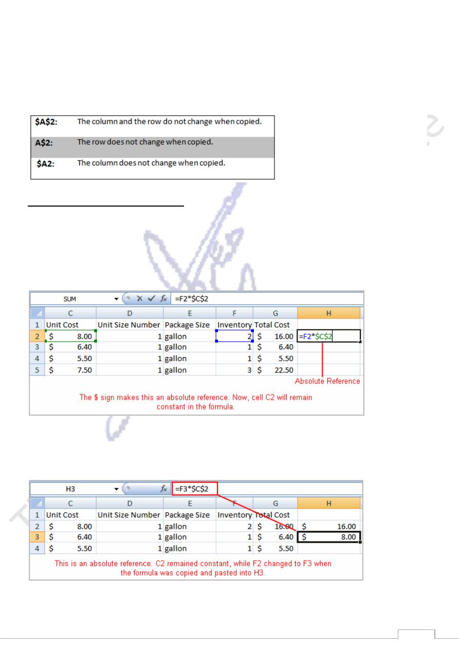
An absolute reference is designated in the formula by the addition of a dollar sign ($). It can precede the
column reference or the row reference, or both. Examples of absolute referencing include:
To Create an Absolute Reference:
Select the cell where you wish to write the formula (in this example, H2)
Type the equal sign (=) to let Excel know a formula is being defined.
Click on the first cell to be included in the formula (F2, for example).
Enter a mathematical operator (use the multiplication symbol for this example).
Click on the second cell in the formula (C2, for example).
Add a $ sign before the C and a $ sign before the 2 to create an absolute reference.
Copy the formula into H3. The new formula should read =F3*$C$2. The F2 reference changed to F3 since it is
a relative reference, but C2 remained constant since you created an absolute reference by inserting the
dollar signs.