116
Each function has a specific order, called syntax, which must be strictly followed for the function to work
correctly.
Syntax Order:
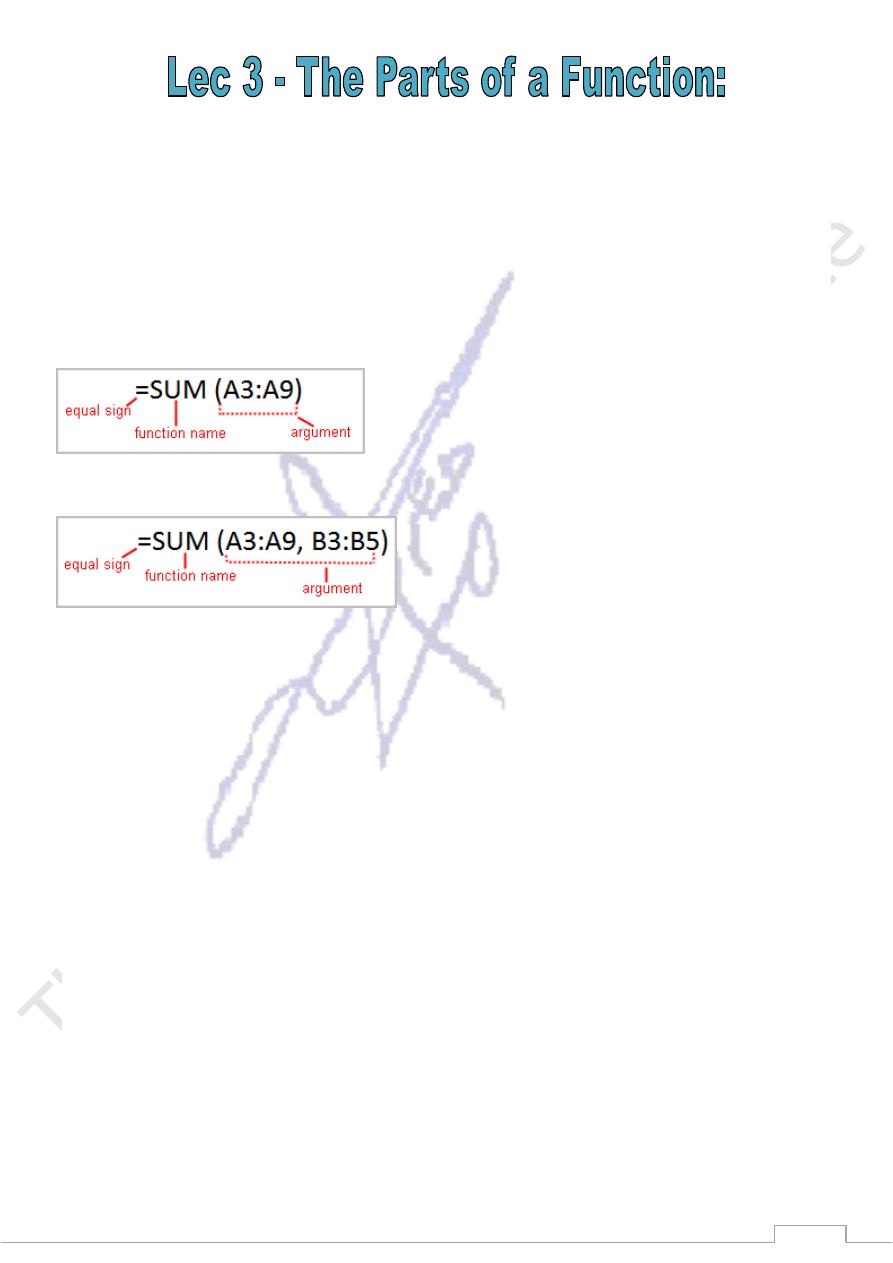
1. All functions begin with the = sign.
2. After the = sign define the function name (e.g., Sum).
3. Then there will be an argument. An argument is the cell range or cell references that are enclosed by
parentheses. If there is more than one argument, separate each by a comma.
An example of a function with one argument that adds a range of cells, A3 through A9:
An example of a function with more than one argument that calculates the sum of two cell ranges:
Excel literally has hundreds of different functions to assist with your calculations. Building formulas can be
difficult and time-consuming. Excel's functions can save you a lot of time and headaches.
Excel's Different Functions
There are many different functions in Excel 2007. Some of the more common functions include:
Statistical Functions:
SUM - summation adds a range of cells together.
AVERAGE - average calculates the average of a range of cells.
COUNT - counts the number of chosen data in a range of cells.
MAX - identifies the largest number in a range of cells.
MIN - identifies the smallest number in a range of cells.
Financial Functions:
Interest Rates
Loan Payments
Depreciation Amounts
117
Date and Time functions:
DATE - Converts a serial number to a day of the month
Day of Week
DAYS360 - Calculates the number of days between two dates based on a 360-day year
TIME - Returns the serial number of a particular time
HOUR - Converts a serial number to an hour
MINUTE - Converts a serial number to a minute
TODAY - Returns the serial number of today's date
MONTH - Converts a serial number to a month
YEAR - Converts a serial number to a year
You don't have to memorize the functions but should have an idea of what each can do for you.
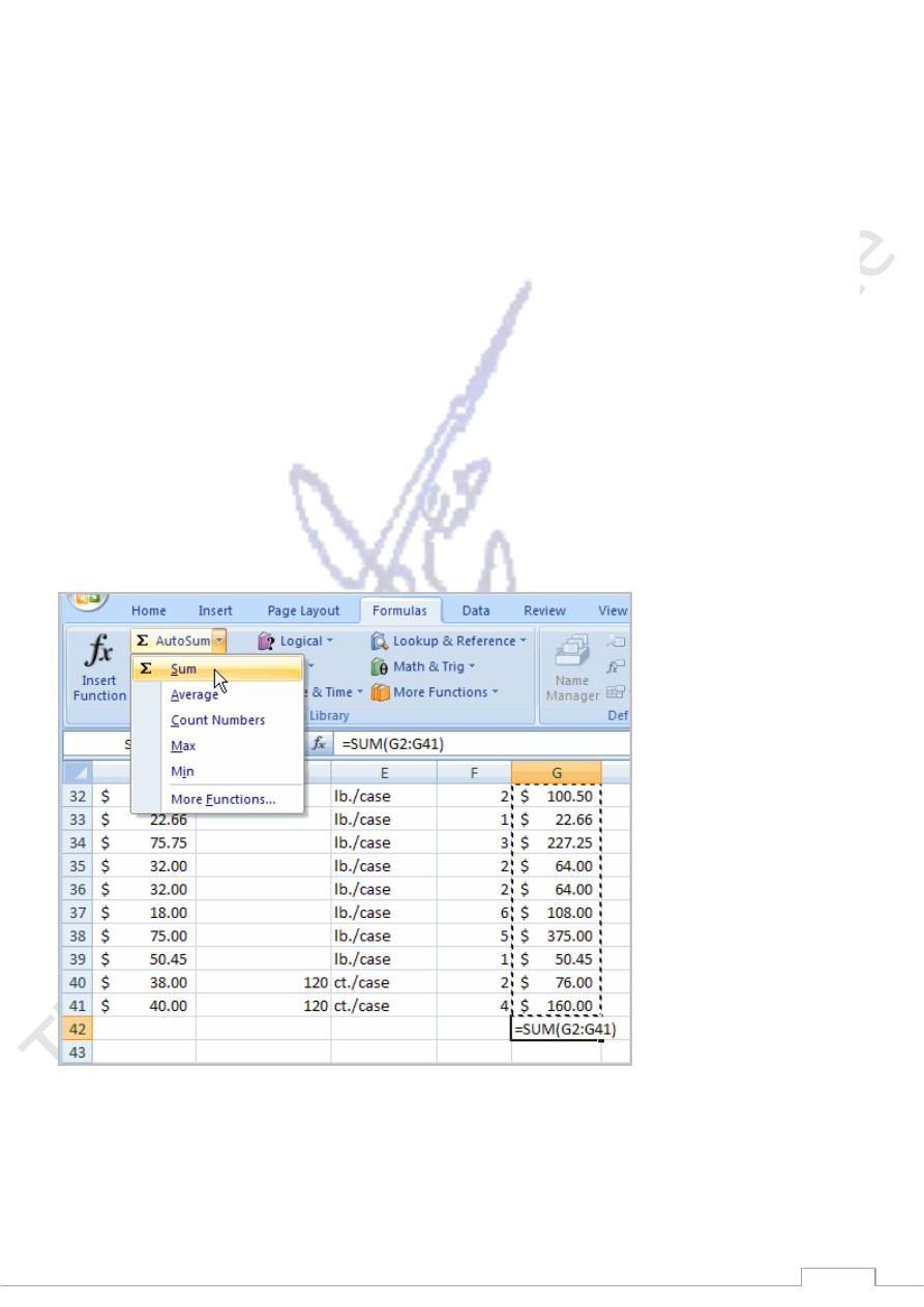
To Calculate the Sum of a Range of Data Using AutoSum:
Select the Formulas tab.
Locate the Function Library group. From here, you can access all the available functions.
Select the cell where you want the function to appear. In this example, select G42.
Select the drop-down arrow next to the AutoSum command.
Select Sum. A formula will appear in the selected cell, G42.
o
This formula, =SUM(G2:G41), is called a function. AutoSum command automatically
selects the range of cells from G2 to G41, based on where you inserted the function. You can
alter the cell range, if necessary.
Press the Enter key or Enter button on the formula bar. The total will appear.
118
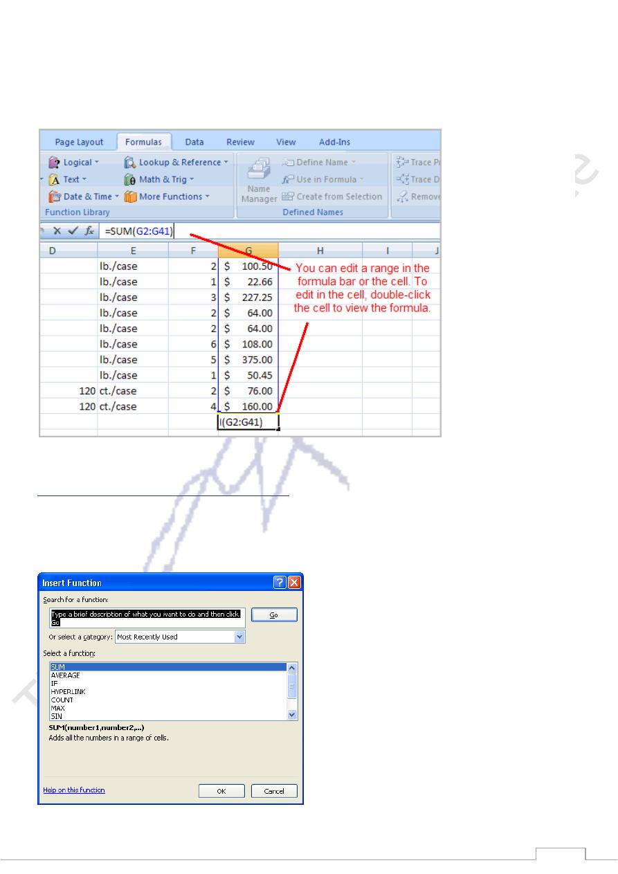
To Edit a Function:
Select the cell where the function is defined.
Insert the cursor in the formula bar.
Edit the range by deleting and changing necessary cell numbers.
Click the Enter icon.
To Calculate the Sum of Two Arguments:
Select the cell where you want the function to appear. In this example, G44.
Click the Insert Function command on the Formulas tab. A dialog box appears.
SUM is selected by default.
119
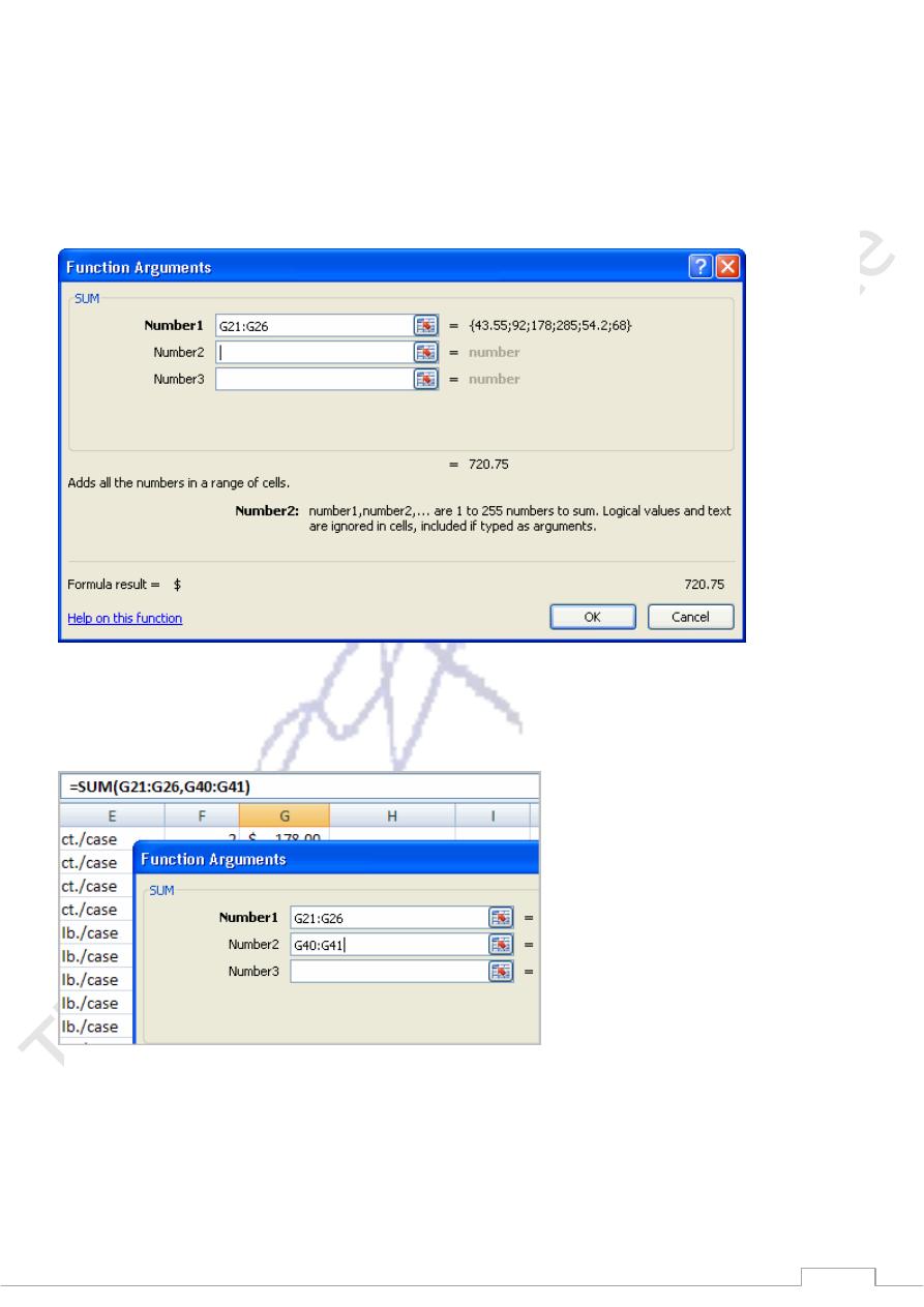
Click OK and the Function Arguments dialog box appears so that you can enter the range of cells
for the function.
Insert the cursor in the Number 1 field.
In the spreadsheet, select the first range of cells. In this example, G21 through G26. The argument
appears in the Number 1 field.
o
To select the cells, left-click cell G21 and drag the cursor to G26, and then release the
mouse button.
Insert the cursor in the Number 2 field.
In the spreadsheet, select the second range of cells. In this example, G40 through G41. The
argument appears in the Number 2 field.
Notice that both arguments appear in the function in cell G44 and the formula bar when G44 is
selected.
Click OK in the dialog box and the sum of the two ranges is calculated.
To Calculate the Average of a Range of Data:
Select the cell where you want the function to appear.
Click the drop-down arrow next to the AutoSum command.
121
Select Average.
Click on the first cell (in this example, C8) to be included in the formula.
Left-click and drag the mouse to define a cell range (C8 through cell C20, in this example).
Click the Enter icon to calculate the average.
Accessing Excel 2007 Functions
To Access Other Functions in Excel:
Using the point-click-drag method, select a cell range to be included in the formula.
On the Formulas tab, click on the drop-down part of the AutoSum button.
If you don't see the function you want to use (Sum, Average, Count, Max, Min), display additional functions
by selecting More Functions.
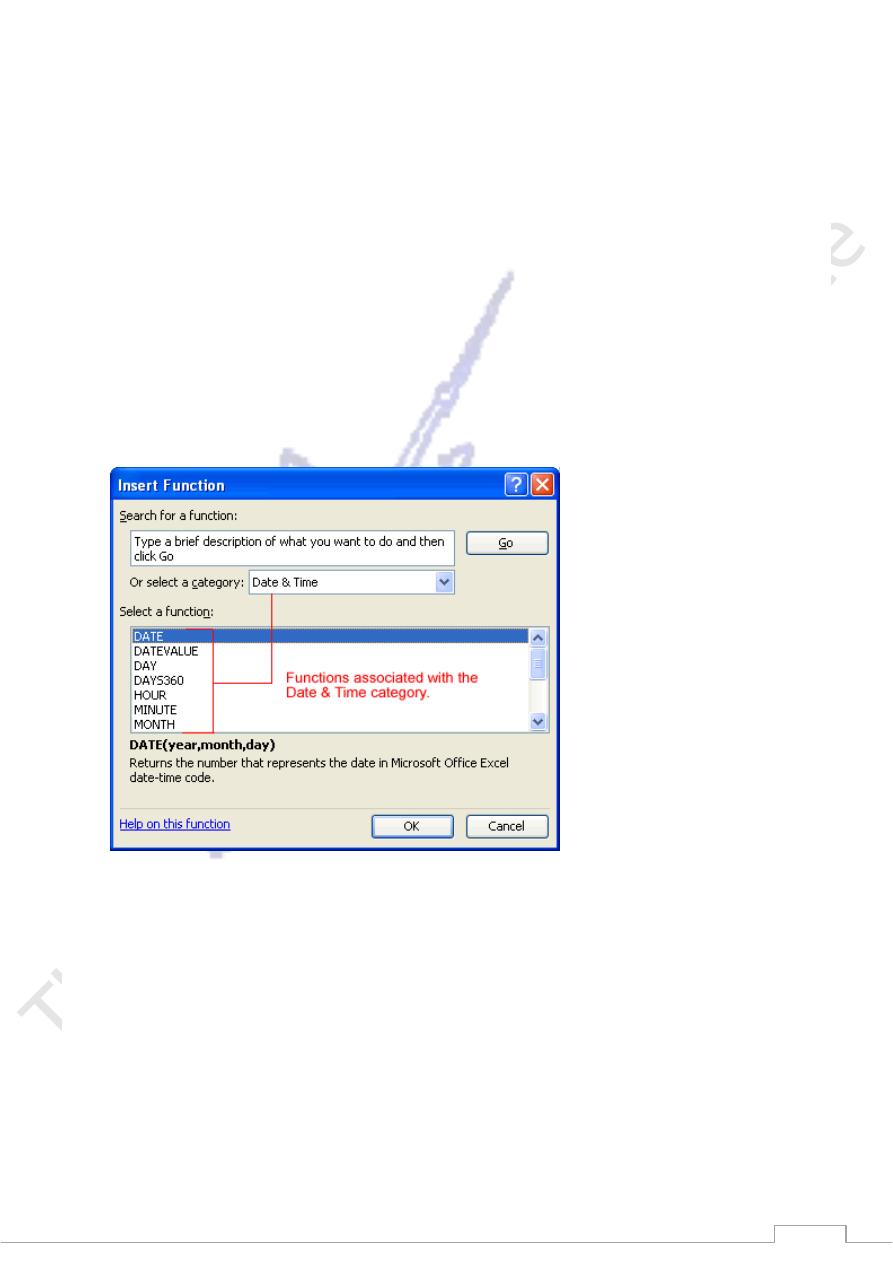
The Insert Function dialog box opens.
There are three ways to locate a function in the Insert Function dialog box:
o
You can type a question in the Search for a function box and click GO, or
o
You can scroll through the alphabetical list of functions in the Select a function field, or
o
You can select a function category in the Select a category drop-down list and review the
corresponding function names in the Select a function field.
Select the function you want to use and then click the OK button.
What-if Analysis
Example
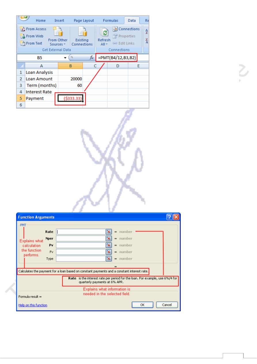
You need a loan to buy a new car. You know how much money you want to borrow, how long of a period
you want to take to pay off the loan (the term), and what payment you can afford to make each month. But
what you need to know is what interest rate you need to qualify for to make the payment $400 a month. In
the image below, you can see that if you didn’t have interest and just divided this $20,000 into 60 monthly
payments, you would pay $333.33 a month. The What-If Analysis tool will allow you to easily calculate the
interest rate.
121
Where Did the Formula Come From?
The formula that appears in cell B5 in the example image is a function. It isn't part of the What-if Analysis
tool, so you will need to understand functions thoroughly before you use What-if Analysis. For the example
scenario described above, you need a formula that will calculate the monthly payment. Instead of writing the
formula yourself, you can insert a function to do the calculation for you.
To Insert a Payment Function:
Select the Formula tab.
Click the Insert Function command. A dialog box appears.
Select PMT.
Click OK. A dialog box appears.
Insert your cursor in the first field. A description about the needed information appears at the bottom
of the dialog box.
Select the cell in the spreadsheet with the needed information.
Insert your cursor in the next field. A description about the needed information appears at the bottom
of the dialog box.
Select the cell in the spreadsheet with the needed information.
Repeat the last two steps until all the necessary information is entered in the dialog box.
122
Click OK.
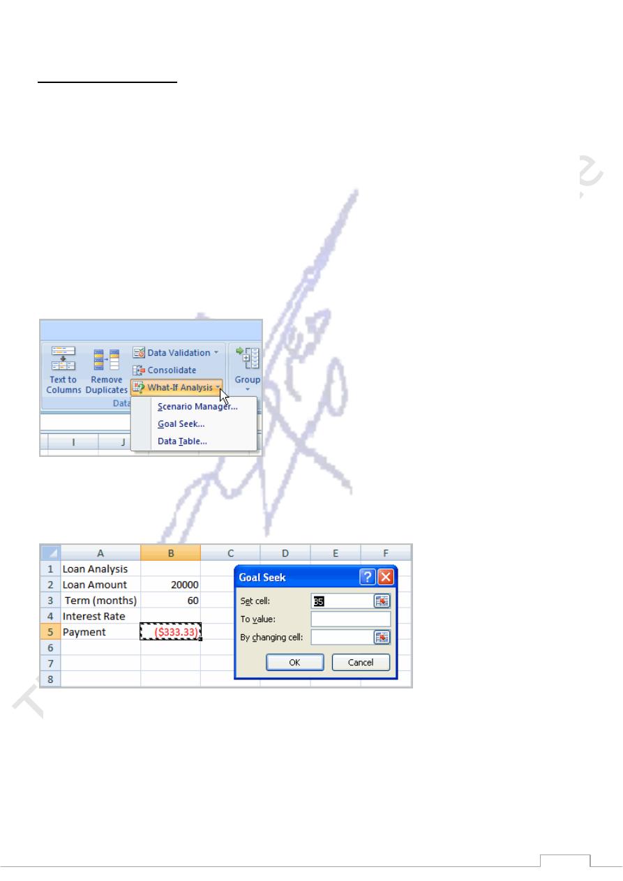
What-If Analysis Tools
There are three What-If analysis tools that you can use. To access these, select the Data tab, and locate the
What-If Analysis command. If you click this command, a menu with three options appears.
Goal seek is useful if you know the needed result, but need to find the input value that will give you the
desired result. In this example, we know the desired result (a $400 monthly payment), and are seeking the
input value (the interest rate).
Goal Seek
To Use Goal Seek to Determine an Interest Rate:
Select the Data tab.
Locate the Data Tools group.
Click the What-If Analysis command. A list of three options appears.
Select Goal Seek. A small dialog box appears.
Select the cell that you what to set to a specific value. In this example, we want to set B5, the
Payment cell.
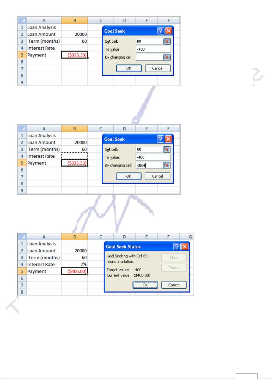
Insert the cursor in the next field.
Enter a value in the value field. In this example, type -$400. Since we’re making a payment that will
be subtracted from our loan amount, we have to enter the payment as a negative number.
123
Insert the cursor in the next field.
Select the cell that you want to change. This will be the cell that tries various input values. In this
example, select cell B4, which is the interest rate.
Click OK.
Then, click OK again. The interest rate appears in the cell. This indicates that a 7% interest rate will
give us a $400 a month payment on a $20,000 loan that is paid off over 5 years, or 60 months.