
Digital Signal Processing (DSP)
1
What is Digital Signal Processing
?
To understand what is Digital Signal Processing (DSP) let's examine what does each of its
words mean.
Signal is any physical quantity that carries information. Processing is a series of steps or
operations to achieve a particular end. It is easy to see that Signal Processing is used
everywhere to extract information from signals or to convert information-carrying signals
from one form to another. For example, our brain and ears take input speech signals, and
then process and convert them into meaningful words. Finally, the word Digital in Digital
Signal Processing means that the process is done by computers, microprocessor, or logic
circuits.
The field DSP has expanded significantly over that last few decades as a result of rapid
developments in computer technology and integrated-circuit fabrication. Consequently,
DSP has played an increasingly important role in a wide range of disciplines in science and
technology. Research and development in DSP are driving advancements in many high-
tech areas including telecommunications, multimedia, medical and scientific imaging, and
human-computer interaction.
Concepts in Digital Signal Processing
The two main characters in DSP are signals and systems. A signal is defined as any physical
quantity that varies with one or more independent variables such as time (one-
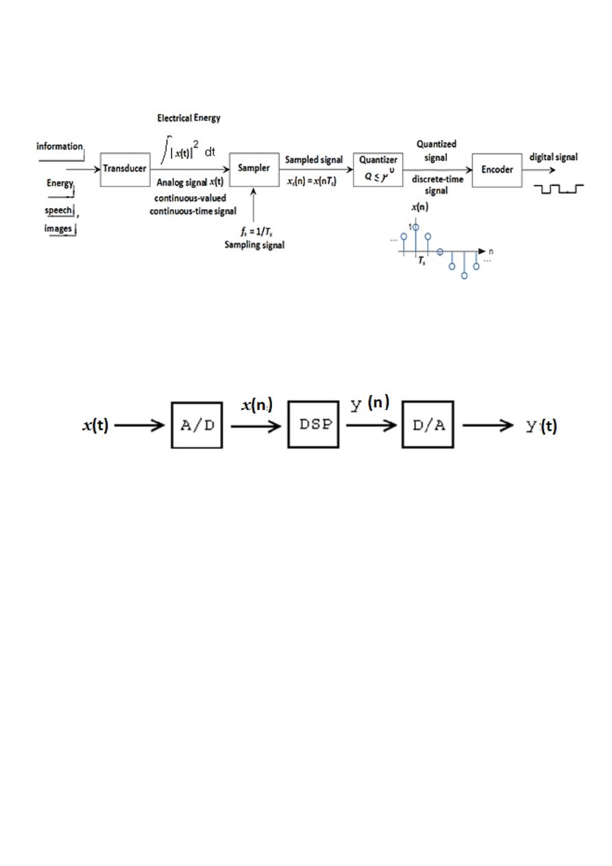
dimensional signal), or space (2-D or 3-D signal). Signals exist in several types. In the real-
world, most of signals are continuous-time (analog signals) those have values continuously
at every value of time. To be processed by a computer, a continuous-time signal has to be
first sampled in time into a discrete-time signal so that its values at a discrete set of time
instants can be stored in computer memory locations. Furthermore, in order to be
processed by logic circuits, these signal values have to be quantized in to a set of discrete
values, and the final coded result is called a digital signal. The terms discrete-time signal
and digital signal can be used interchangeability to define two different formats (Fig. 1).
In signal processing, a system is defined as a process coder whose input and output are
signals (Fig. 2).
Signals Represent Information
Whether analog or digital, information
is represented by the fundamental quantity in
electrical engineering: the signal. Stated in mathematical terms, a signal is merely a
function. Analog signals are continuous-valued; digital signals are discrete-valued. The
independent variable of the signal could be time (speech), space (images), or the integers
(denoting the sequencing of letters and numbers in the football score).
Digital Signal Processing (DSP)
2
Fig. 1
Fig. 2

Digital Signal Processing (DSP)
3
Sampling
Why sample? Sampling is the necessary fundament for all digital signal processing and
communication. Sampling can be defined as the process of measuring an analog signal at
distinct points. Digital representation of analog signals offers advantages in terms of
1-Robustness towards noise, meaning we can send more bits/s.
2-Use of flexible processing equipment, in particular the computer.
3-More reliable processing equipment.
4-Easier to adapt complex algorithms.
Claude Shannon has been called the father of information theory, mainly due to his
landmark papers on the "Mathematical theory of communication". Harry Nyquist was the
first to state the sampling theorem in 1928, but it was not proven until Shannon proved it
21 years later in the paper "Communications in the presence of noise".
The following notations will be used: Original analog signal x(t), Sampling frequency
f
s
,
Sampling interval T
s
(Note that: f
s
= 1/T
s
), Sampled signal x
s
(n). (Note that x
s
(n) = x(nT
s
),
Analogue angular frequency Ω , and Digital angular frequency ω (Note that: ω = Ω T
s
).
The Sampling Theorem
[[When sampling an analog signal the sampling frequency must be greater than twice the
highest frequency component of the analog signal to be able to reconstruct the original
signal from the sampled version]].
The process of sampling
We start with an analog signal. This can for example be the sound coming from your
stereo at home or your friend talking. The signal is then sampled uniformly. Uniform
sampling implies that we sample every T
s
seconds. In Fig. 3, we see an analog signal. The
analog signal has been sampled at times t = nT
s
.
Digital Signal Processing (DSP)
4
Fig. 3
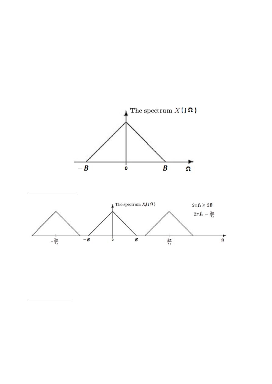
In signal processing it is often more convenient and easier to work in the frequency
domain. So let's look at the signal in frequency domain, Fig. 4 . For illustration purposes we
take the frequency content of the signal as a triangle. (If you Fourier transform the signal
in Fig. 3 you will not get such a nice triangle.)
Fig. 4
Sampling fast enough
Fig. 5
From Fig. 5, and according to the sample theorem, an aliasing-free condition appears. So,
we are able to reconstruct the original signal exactly. How can we do this? will be explored
further down under reconstruction. But first we will take a look at what happens when we
sample too slowly.
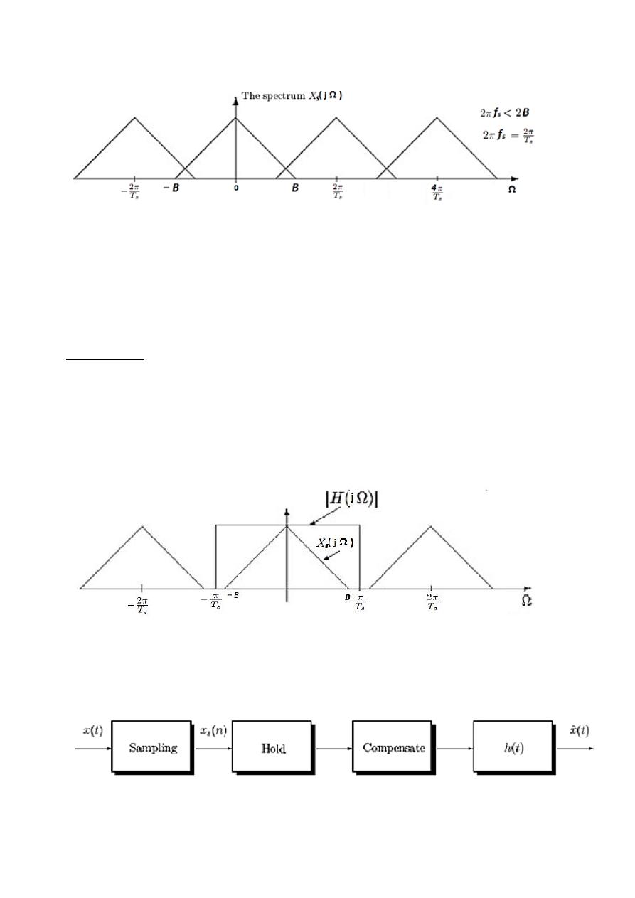
Sampling too slowly
We will get overlap between the repeated spectra, see Fig. 6. The resulting spectra is the
sum of these. This overlap gives rise to the concept of aliasing.
Digital Signal Processing (DSP)
5
Fig. 6
To avoid aliasing we have to sample fast enough. But if we can't sample fast enough
(possibly due to costs) we can include an Anti-Aliasing filter. This will not able us to get an
exact reconstruction but can still be a good solution.
Note: Typically a low-pass filter that is applied before sampling to ensure that no
components with frequencies greater than half the sample frequency remain.
Reconstruction
We want to recover the original signal, but the question is how?
The Answer: By using a simple reconstruction process. To achieve this we have to remove
all the extra components generated in the sampling process. To remove the extra
components we apply an ideal analog low-pass filter as shown in Fig. 7. As we see the ideal
filter is rectangular in the frequency domain. A rectangle in the frequency domain
corresponds to a sinc function in time domain (and vice versa).
Fig. 7
Digital Signal Processing (DSP)
6
Digital Signal Processing (DSP)
7
( ) ∑
( ) ( ) ( ) ( )
Digital Signal Processing (DSP)
8
Digital Signal Processing (DSP)
9
Digital Signal Processing (DSP)
11
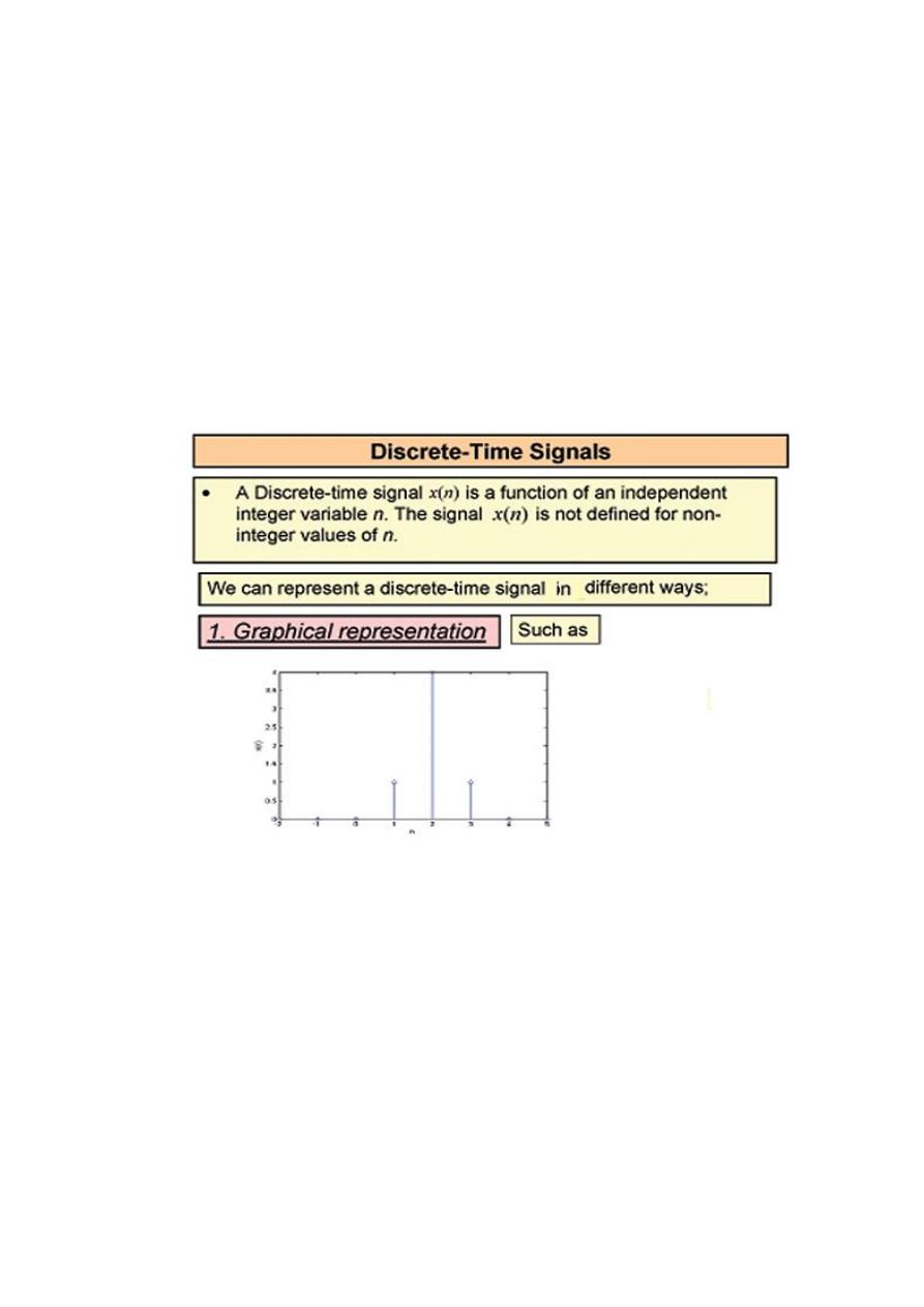
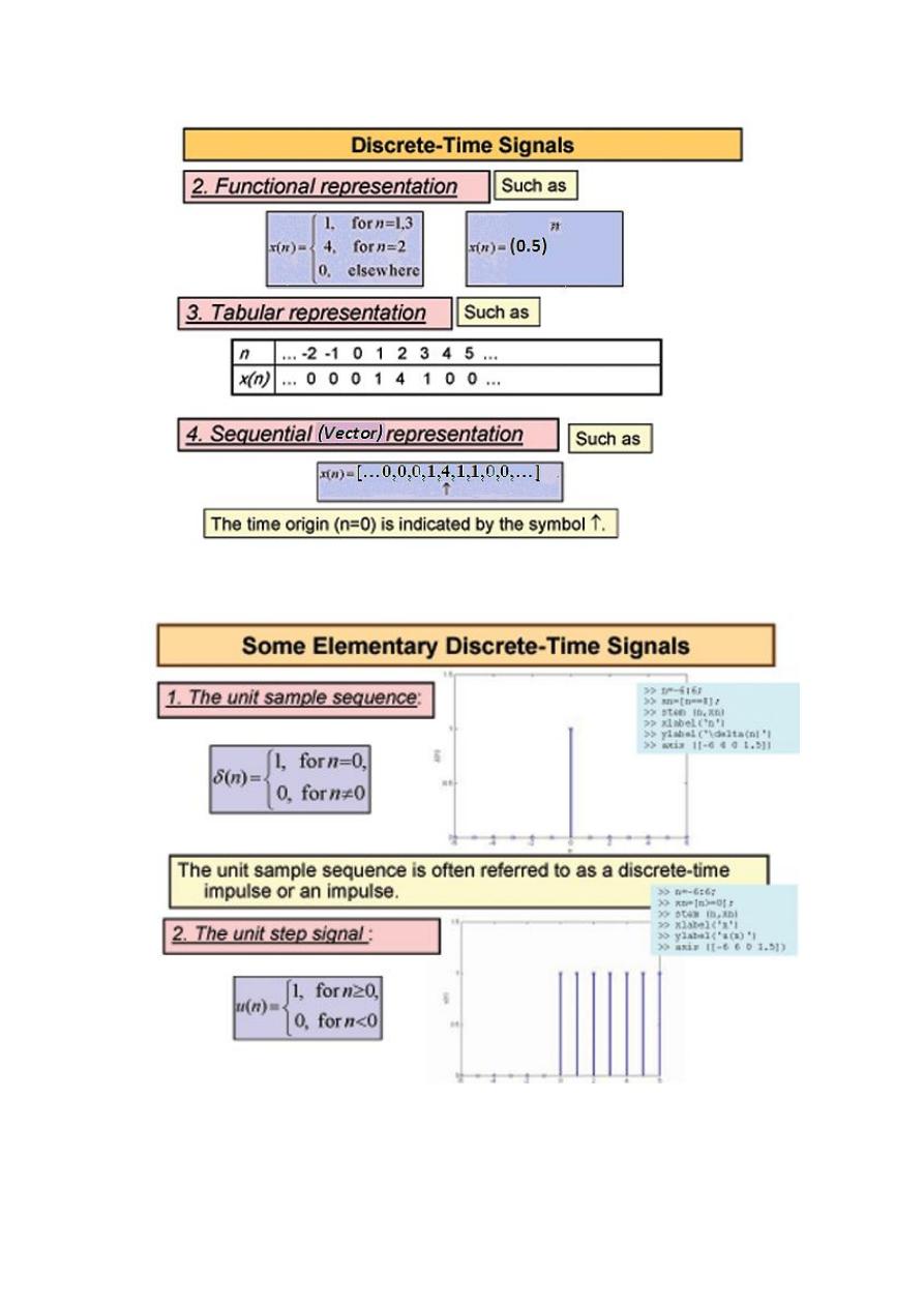
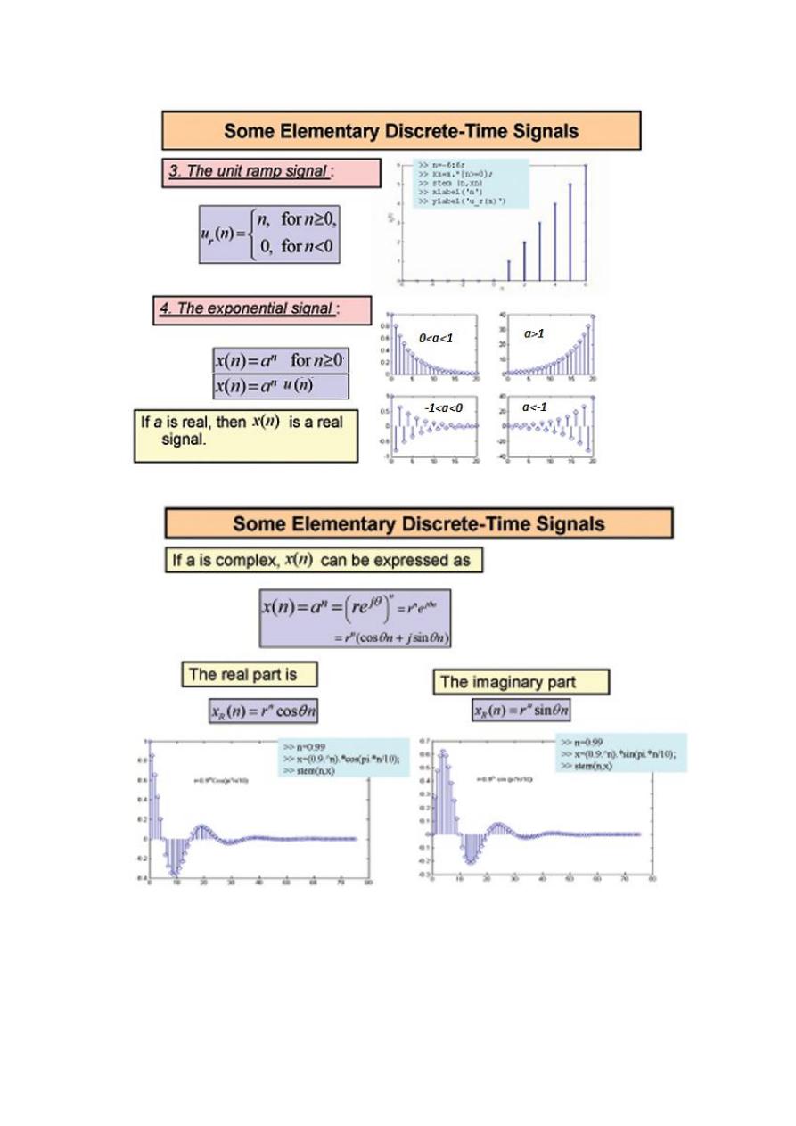
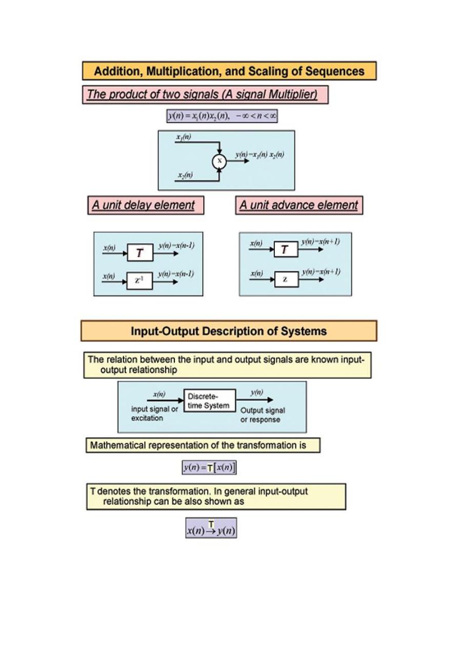
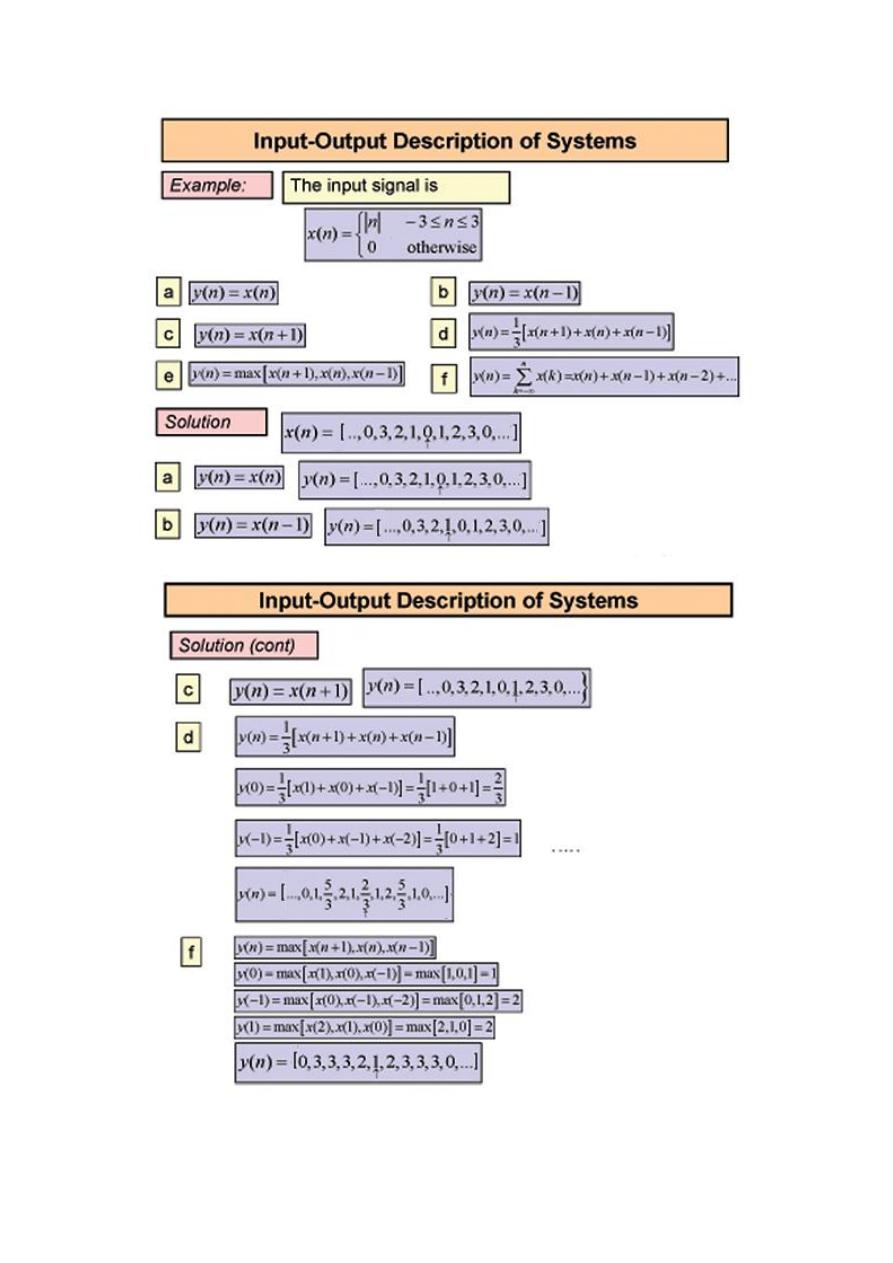
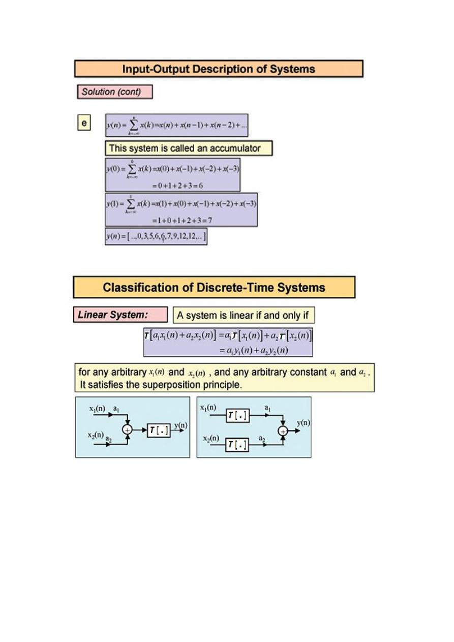
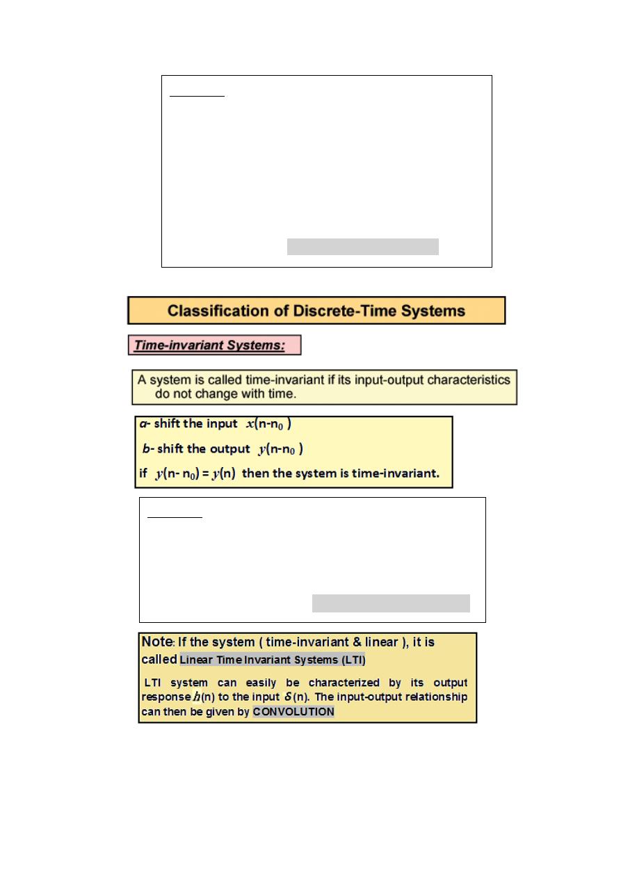
Discrete-Time Signals and Systems
Digital Signal Processing (DSP)
11
Digital Signal Processing (DSP)
12
Digital Signal Processing (DSP)
13
( )
( )
( )
( )
,
( )
( )- ( )
( ) ,
( )
( )-
Digital Signal Processing (DSP)
14
( ) ( ) ( ) ∑ ( ) ( )
( )
( )
( )
( )
,
( )
( )- ( )
,
( )
( )-
,
( )
( )-
( )
( )
,
( )
( )-
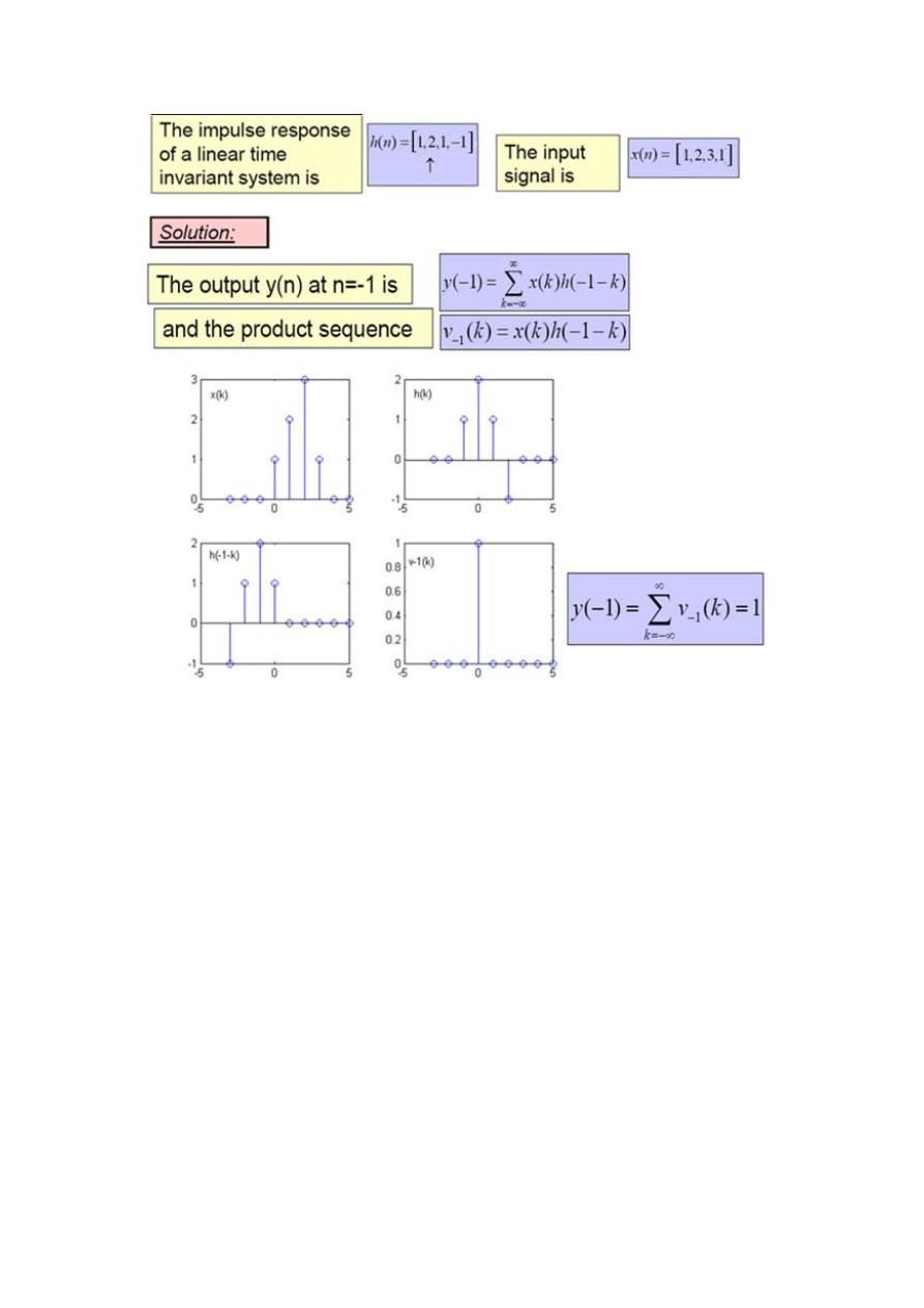
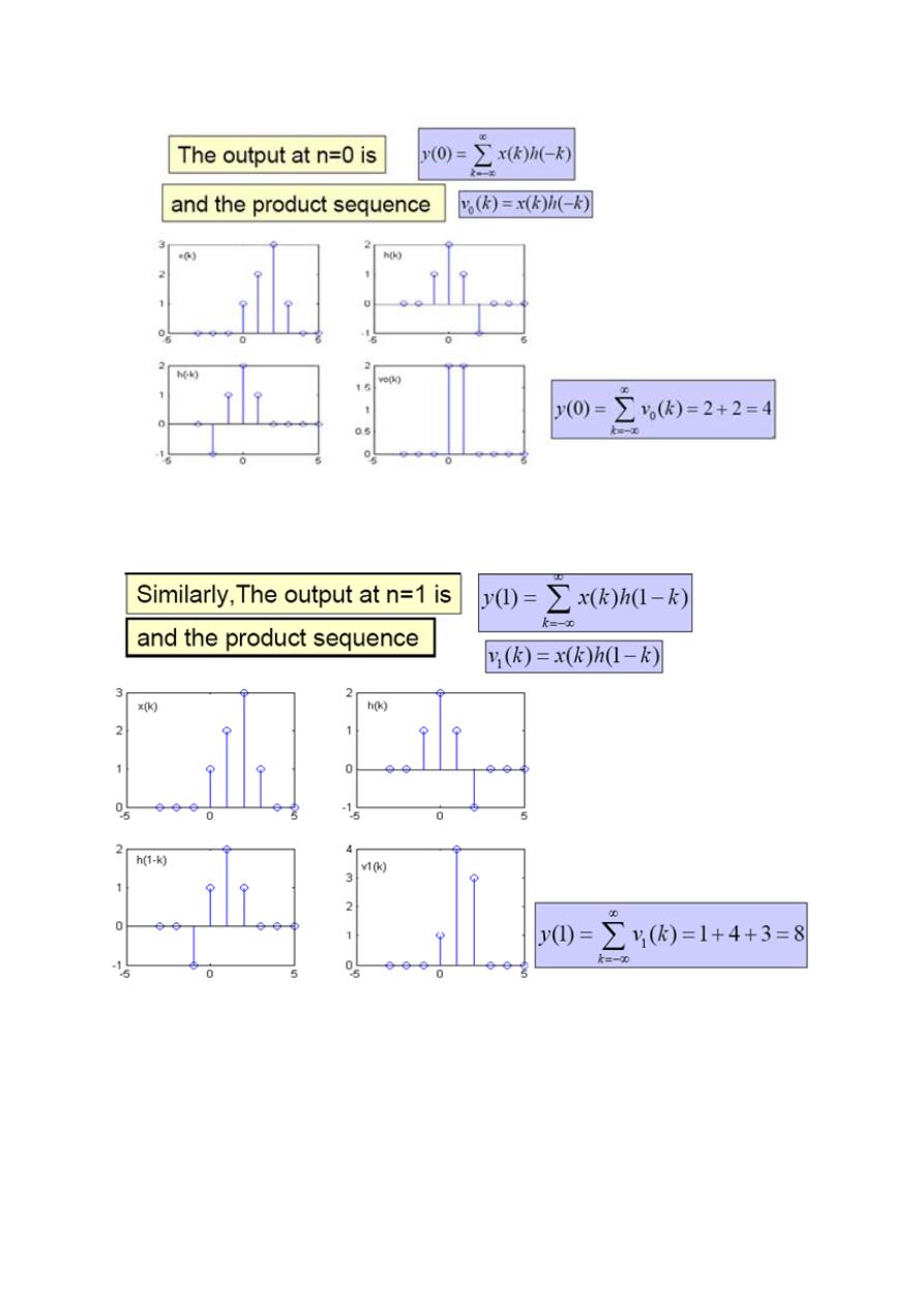
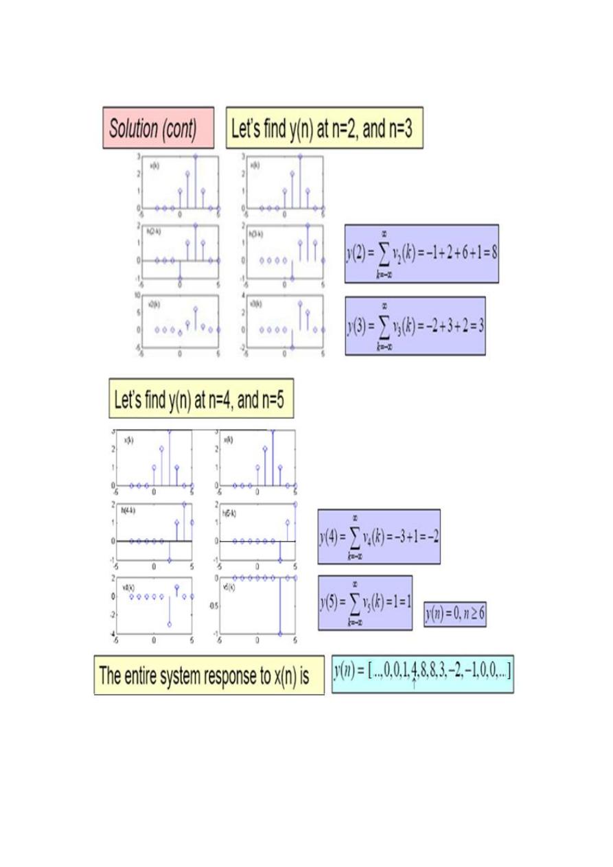
Example 1:
( )
( )
Example 2
:
y
(n)=n x(n -1)
: Shift the input, y(n)=n x(n- n
0
-1)
shift the output, y(n- n
0
)= (n- n
0
) x(n- n
0
-1)
since y(n- n
0
) y(n) , then the system is time-variant.
Digital Signal Processing (DSP)
15
Example 3
: y(n)= x(n+1)
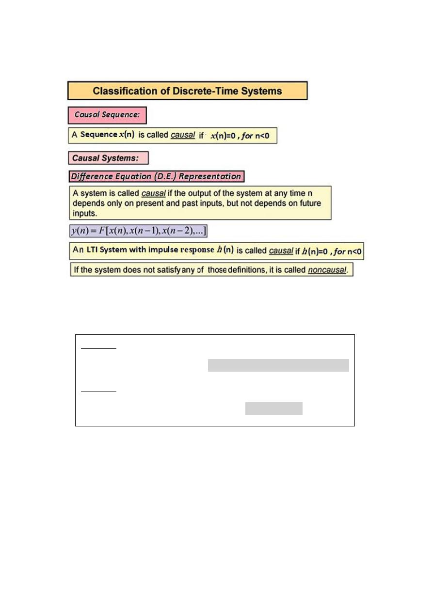
At n = 0, y(0) = x(1), then the system is non-causal (anti-causal).
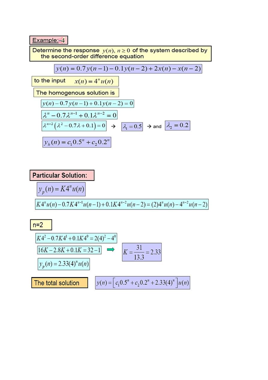
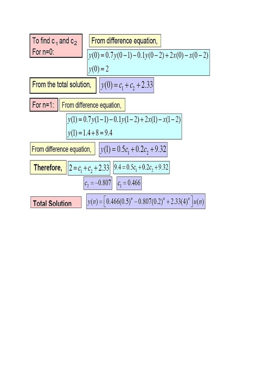
Example 4
: ( )
( )
Since ( ) , then it is a causal system
Digital Signal Processing (DSP)
16
Example 5
: y(n)= n x(n-1)
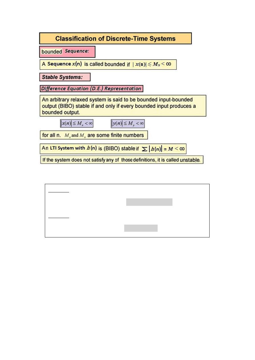
As n → , y(n) → , then the system is unstable.
Example 6
:
( ) (
⁄ )
( )
Since ∑
| ( )|
, it is a stable system
Digital Signal Processing (DSP)
17
Digital Signal Processing (DSP)
18
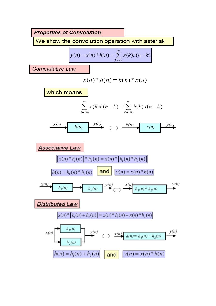
Convolution

Digital Signal Processing (DSP)
19
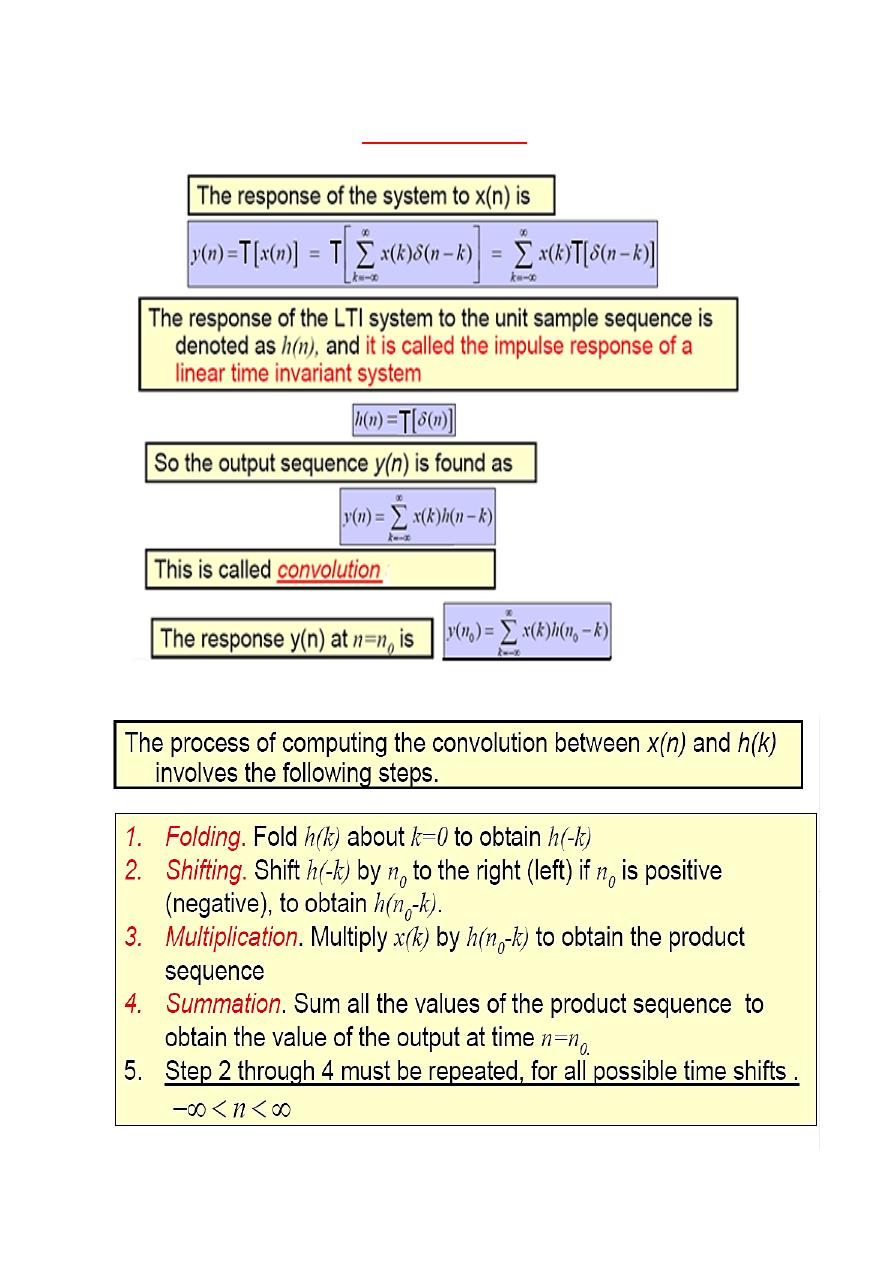
Methods of Convolution
1- Graphical method.
2- Table-look up method.
3- Vector-by-matrix method.
4- Add-overlap method.
5- Analytical method.
1- Graphical Method
Digital Signal Processing (DSP)
21
Digital Signal Processing (DSP)
21
Digital Signal Processing (DSP)
22
Digital Signal Processing (DSP)
23
Digital Signal Processing (DSP)
24
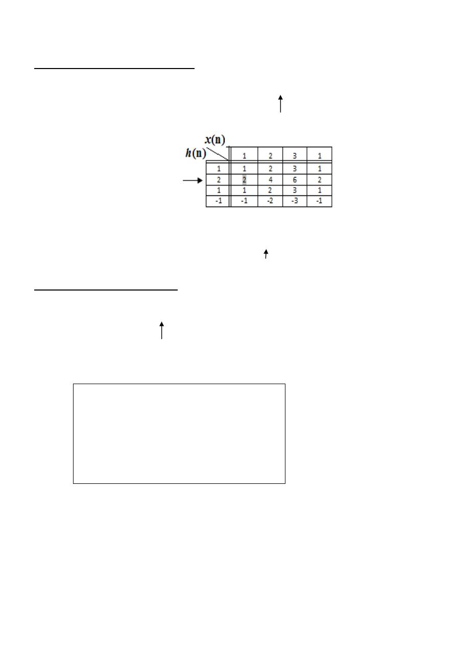
2- Table-look up Method h(n)
( ) , - ( ) , -
( )
( )
, -
3- Vector-by-matrix Method
( ) , - ( ) , -
( )
22
[
]
[
]
[
]
Digital Signal Processing (DSP)
25
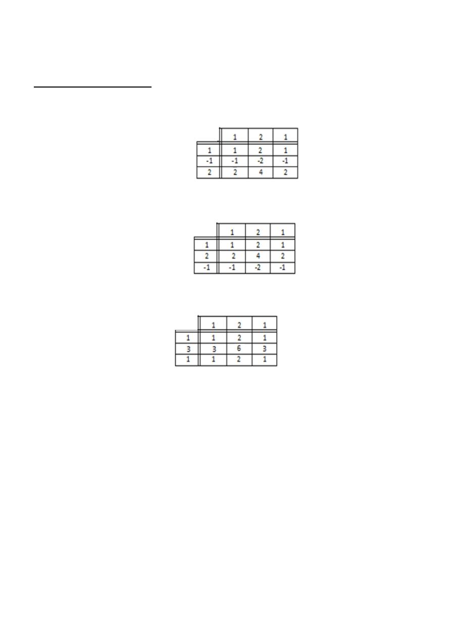
4- Add-overlap Method
( ) , - ( ) , -
( )
, -
( )
, -
( )
, -
( )
[
]
( )
[
]
( )
, -
( )
( )
( )
( )
( )
, -

Digital Signal Processing (DSP)
26
5- Analytical Method
( ) ∑
( ) ( )
( )
( )
( ) ∑
( ) ( )
How to calculate
and
?
( )
( )
*
+
*
+
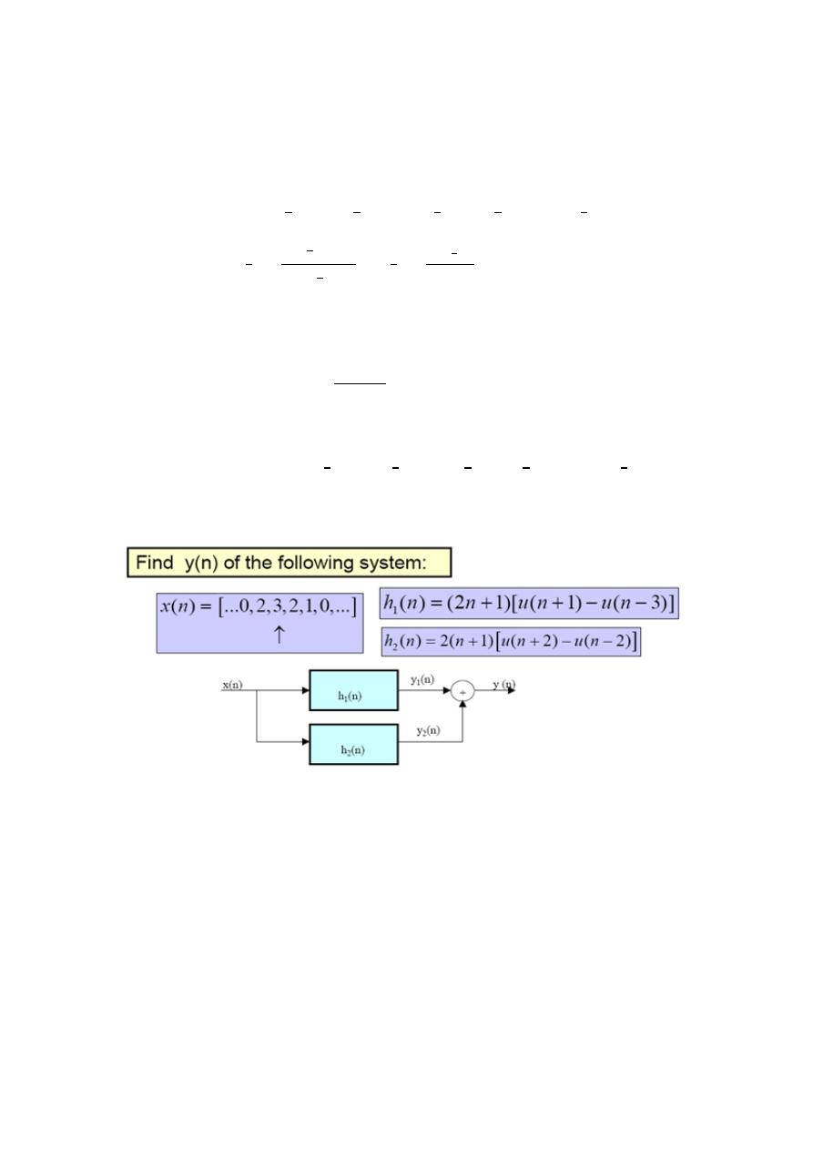
Example:
( ) ( ) ( ) ( ) ( )
.
/
( )
Solution:-
N
1
=0 , N
2
=9
M
1
=0 M
2
=
*
+ *
+
*
+
*
+
*
+
2
Digital Signal Processing (DSP)
27
( )
∑
( ) ( ) ∑
.
/
.
/
∑
.
/
.
/
∑
[.
/
]
.
/
[
[.
/
]
.
/
]
.
/
[
0.
/1
]
The last step above is obtained by using the geometrical progression formula given in appendix B (
page 317 in ( fundamentals of digital signal processing book) by
∑
( )
0
( )
1
( ) ∑
( ) ( ) ∑
.
/
.
/
[ .
/
.
/
.
/
]
H.W

Digital Signal Processing (DSP)
28
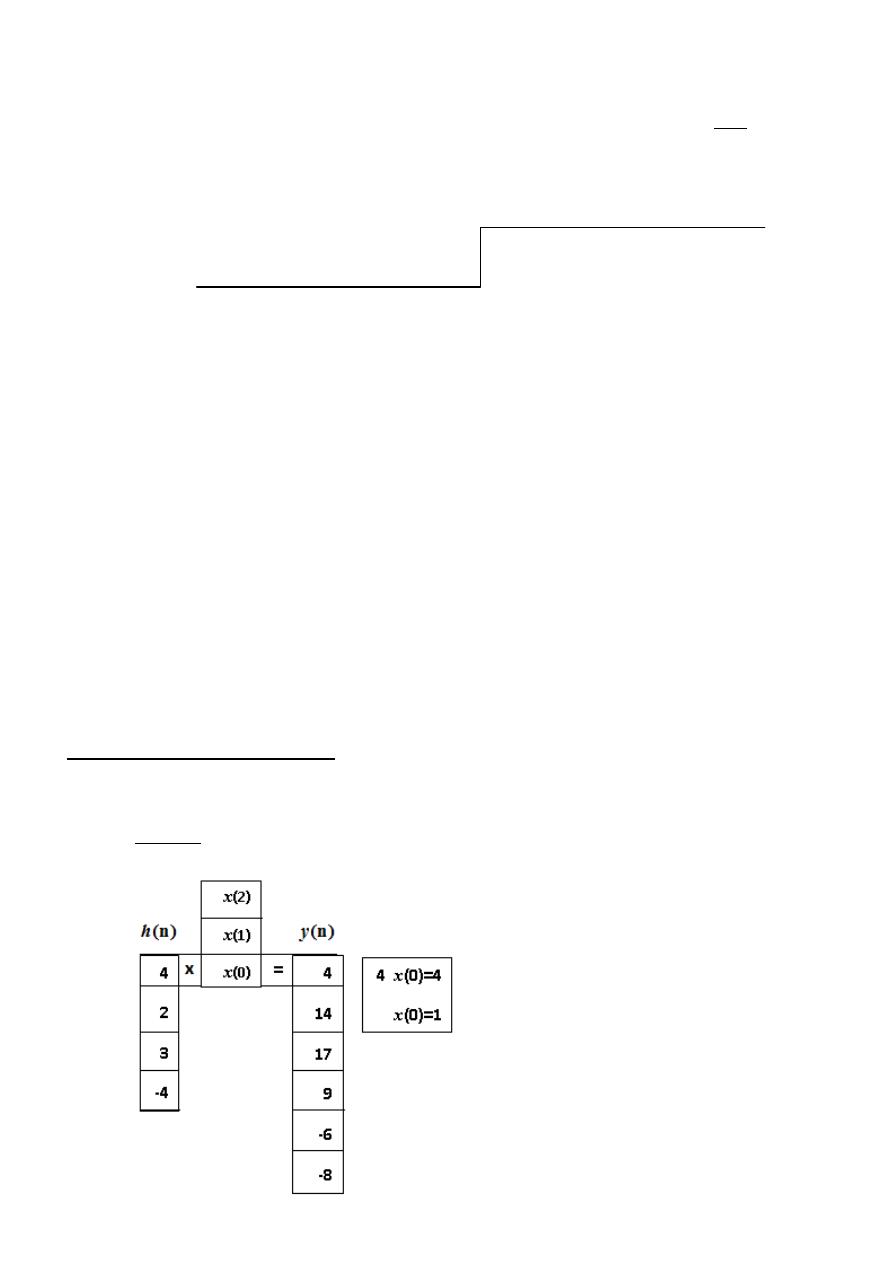
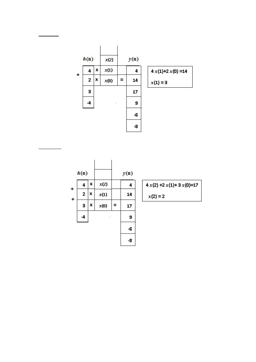
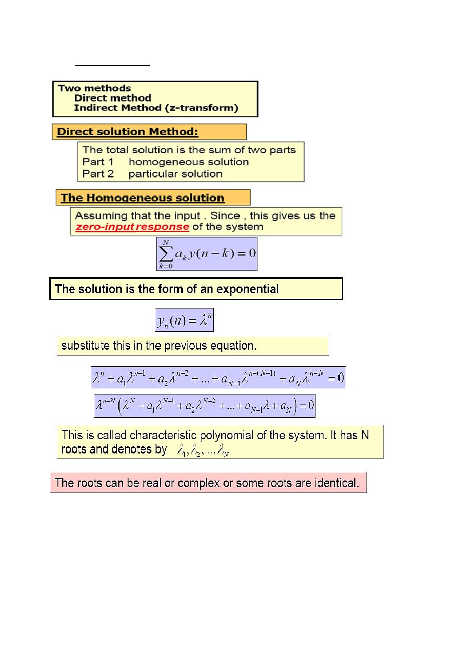
De-convolution
1-Iterative method
Example:
( ) , - ( ) , -
( )
( ) ∑
( ) ( )
( ) ∑
( ) ( )
( ) ( )
( )
( )
( )
( ) ∑
( ) ( )
( ) ( )
( ) ( )
( )
( ) ( ) ( )
( )
(
)
( ) ∑
( ) ( )
( ) ( )
( ) ( )
( ) ( )
( )
( ) ( ) ( )
( ) ( )
( )
(
)
(
)
( ) ∑
( ) ( )
( ) ( )
( ) ( )
( ) ( )
( ) ( )
( )
( ) ( ) ( )
( ) ( )
( ) ( )
( )
( ) ( ) ( )
( )
( )
then
(
)
(
)
For the above example, N = 3,and M = 4, then ( )
2-The Polynomial Method
Example:
( ) , - ⇒ ( )
( ) , - ⇒ ( )
Digital Signal Processing (DSP)
29
Since ( ) ( ) ( ) then ( ) ( ) ( ) or ( )
( )
( )
3-The Graphical Method
For the same example:
( ) , -
and ( ) , -
STEP ONE
Digital Signal Processing (DSP)
31
STEP TWO
STEP THREE
If we calculate x(3) and so on, they will be zero. Why?

Digital Signal Processing (DSP)
31
Linear Constant-Coefficient Difference Equations (LCCDEs)
Remembering linear differential equations
( )
( ) ( )
A difference equation is the discrete-time analogue of a differential equation.
We simply use differences [ x (n) - x (n-1)] rather than derivatives (
( )
).
An important subclass of linear systems are those whose input is
x(n)
, output
is
y(n)
, and satisfying the following N
th
- order LCCDE:
∑
( )
∑
( )
If the system is causal, then we can rearrange the above Eq. as
( ) ∑
( )
∑
( )
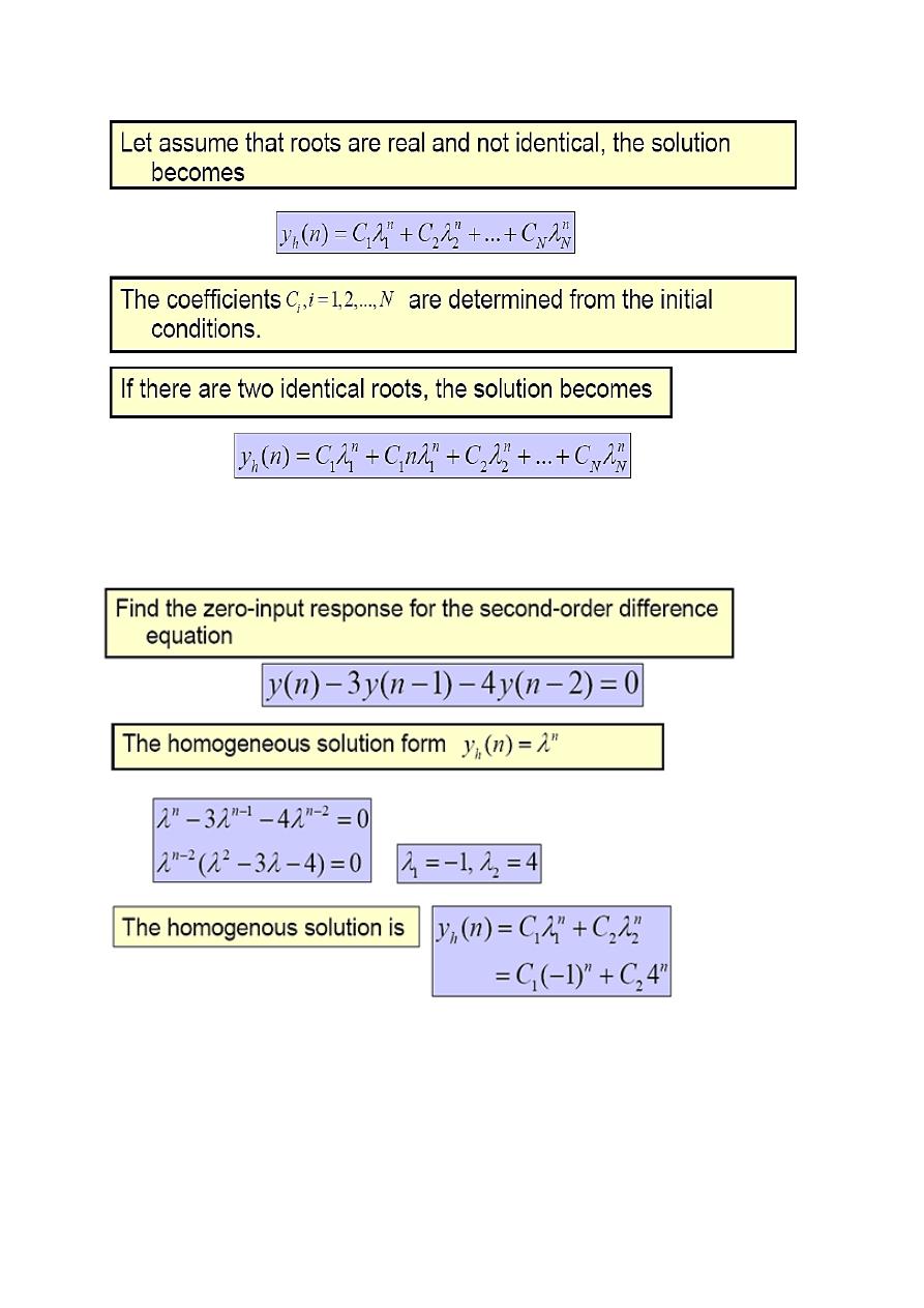
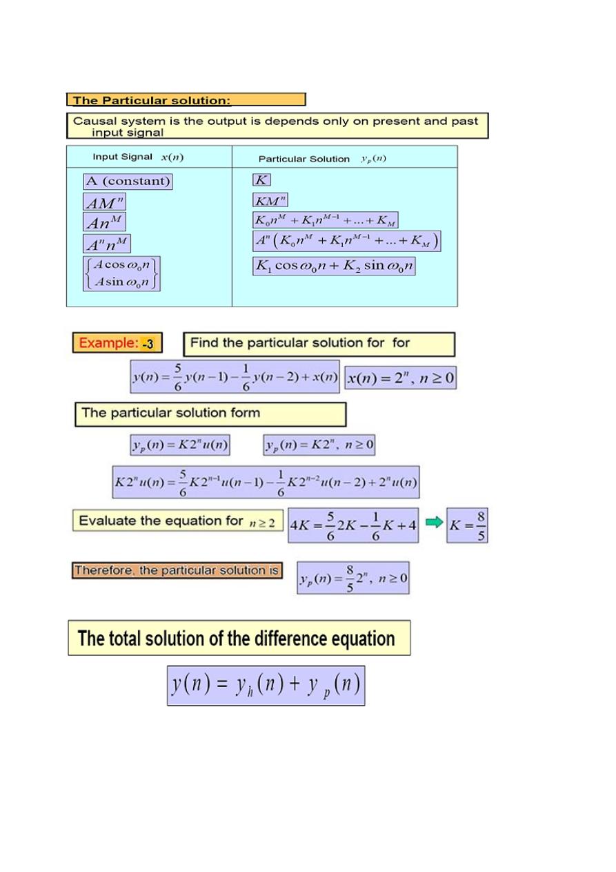
Solutions of Linear Constant- Coefficient Difference Equations
First -order LCCDE
Example -1: Solve the following DE for y (n), assuming y (n) = 0 for all n < 0
and x (n)= δ (n).
y (n) − ay (n − 1) = x (n)
This corresponds to calculating the response of the system when excited by
an impulse, assuming "zero initial conditions"
Solution: Rewrite
( ) ( ) ( )
Evaluate:
( ) ( ) ( )
( ) ( ) ( )
( ) ( ) ( )
For all n>0, It can be written that
( )
Since the response of the system for n < 0 is defined to be zero, the unit
sample response becomes
( )
( )
If
| |
, then the system is …………………?
If
| |
, then the system is …………………?
Digital Signal Processing (DSP)
32
N
th
-order LCCDE
Digital Signal Processing (DSP)
33
Example-2:
Digital Signal Processing (DSP)
34
Digital Signal Processing (DSP)
35
Digital Signal Processing (DSP)
36

Digital Signal Processing (DSP)
37
Frequency Response of LTI Systems
The Fourier representation of signals plays an extremely important role in both
continuous-time and discrete-time signal processing. It provides a method for
mapping signals into another "domain" in which to manipulate them. What makes the
Fourier representation particularly useful is the property that the convolution
operation is mapped to multiplication. In addition, the Fourier transform provides a
different way to interpret signals and systems. In this section, we will develop the
discrete-time Fourier transform (i.e., a Fourier transform for discrete-time signals).
We will show how complex exponentials of linear time-invariant (LTI) systems and
how this property leads to the notion of a frequency response representation of LSI
systems.
A. Response to Complex Exponential
Let
( )
be input into an LTI system with causal impulse response h(n).
The output is
( ) ( ) ( ) ( )
∑
( ) ( )
∑
( )
( )
∑
( )
Let us define
(
): a function of , as varies form ( )
to be
(
) ∑
( )
( )
(
)
or
( ) ( ) (
)
•
(
)
= frequency response function (a conjugate symmetric function of
)
(
)
(
)
(
) | (
)|
(
)
| (
)|
(
)
•
|
.
/|
= Magnitude response (an even function of
)
•
(
)
=
(
)
= Phase response (an odd function of
)
•
(
)
is periodic with period =
where the magnitude and phase of
(
)
are given by
| (
)| [
(
)
(
)]
(
) (
)
[
(
)
(
)
⁄
]

Digital Signal Processing (DSP)
38
B. Response to Sinusoidal
Now let
( ) (
)
be
input into an LTI system with causal impulse response h(n).
Because of linearity the response can be found by adding the responses of the
complex exponential sequences of
and
the output
becomes
( ) (
)
⁄ (
)
⁄
The second part of y(n) is seen to be the complex conjugate of the first part, thus
y(n) becomes two times the real part of either; that is
( ) [
(
)
]
( ) [
| (
)|
(
)
]
( ) 2| (
)|
, (
(
))-
3
( ) | (
)| (
(
))
Therefore, it has been shown that the output to sinusoid is another sinusoid of the
same frequency but with different phase and different magnitude.
Example -1:- Find the frequency response of LTI system characterized by
unit sample response (impulse response)
( )
( ) | |
Solution:
It is an IIR system
By definition the frequency response
(
) is given by
(
) ∑ ( )
∑
∑
(
)
=
( ) ( )
Mag. response
|
(
)|
,( )
( )
-
(
)
Phase response
(
)
, ( )
⁄
-
Change in
phase
Change in
magnitude
Digital Signal Processing (DSP)
39
Plot
Mag. and Phase responses for
Example -2:- For an LTI discrete-time system with the following impulse response
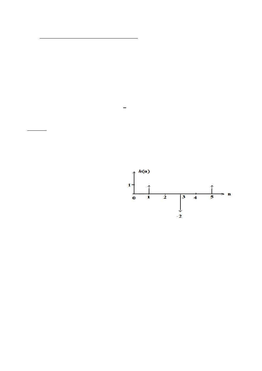
h(n) = δ(n – 1) – 2 δ(n – 3) + δ(n – 5)
(i) Give expressions for h(n) in terms of unit steps and then in vector form.
(ii) Plot such impulse response h(n).
(iii) Specify whether the system is of the FIR or of the IIR type, Why?
(iv) Find the frequency response H(e
jω
).
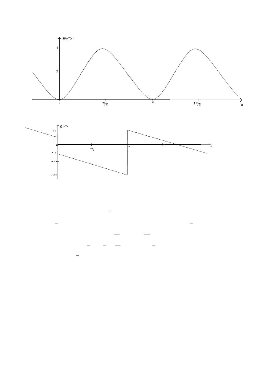
(v) Find and plot magnitude and phase responses.
(vi) Compute the unit step response.
(vii) Compute the response to x(n) = 4 cos[
( n – 2)] . Then calculate the corresponding
time delay of the system if the sampling rate is 8 k sample/sec.
Solution:
(i) Using the fact that a unit sample can be written as the difference of two steps as follows:
(n) = u(n) – u(n – 1)
Therefore, h(n) = [ u(n – 1) – u(n – 2)] – 2[ u(n – 3) - u(n - 4)] + [ u(n – 5) - u(n – 6)]
i.e., h(n) = u(n – 1) - u(n – 2) – 2 u(n – 3) + 2 u(n - 4) + u(n – 5) - u(n – 6)
In vector form,
h(n) = [ 0 1 0 – 2 0 1]
(ii) The plot of such
impulse response
h(n)
is shown here
.
(iii) The system is of the FIR type, because h(n) is of finite duration.
(iv) H(e
jω
)
=
∑
( )
=
=
,
- =
, ( )-
=
( ) , ( )- =
(
) , ( )-
=
( )
, ( )-
(v) From the above frequency response,
Magnitude response =
| (
)| =
, ( )-
.
Phase response =
(
)
( 3
ω
+
)
3
ω
Digital Signal Processing (DSP)
41
(vi)
The unit step response is u(n) * h(n) = u(n) * [ δ(n – 1) – 2 δ(n – 3) + δ(n – 5) ]
= u(n – 1) – 2 u(n – 3) + u(n – 5)
.
(vii)
The response to x(n) = 4 cos[
( n – 2)]
ω
0
=
, So
| (
)| =
, (
)- =0 .
/1 .
(
)
3 ω
0
=
=
y(n) = 4 . (
) .
cos[
n –
)] =
.
cos[
(n –
)]
=
.
cos[
(n
)]
Delay = 9
2=7
samples, Time delay = 7 T
s
= 7/f
s
= 7/8000 = 0.000875 sec.
= 0.875 m sec.

Digital Signal Processing (DSP)
41
Example -3:- If the step response of an LTI system is
y
u
(n) = [ 1 3 2 2 3 1],
find the unit sample response h(n). Then find magnitude and phase
responses. Is the system possesses a linear phase response? Plot it.
Solution:
It is known that
(n) = u(n) –u (n – 1), So
h(n) *
(n) = h(n) * [u(n) – u (n – 1)]
or h(n) *
(n) = h(n) * u(n) – h(n) * u (n – 1),
i.e., h(n) = y
u
(n) - y
u
(n – 1) =
[ 1 3 2 2 3 1 0] - [0 1 3 2 2 3 1]
h(n) = [1 2 -1 0 1 -2 -1]
H(
) = 1 + 2
–
+ 0 .
+
– 2
–
H(
) =
[ (
–
) + 2 (
–
)
–
(
–
) ]
H(
) =
[ 2
sin(
) + 4
sin(
)
–
2
sin(
) ]
H(
) =
[ 2 sin(
) + 4 sin( )
–
2 sin(
) ]
H(
) =
[ 2 sin(
) + 4 sin( )
–
2 sin(
) ]
H(
) =
(
)
[ 2 sin(
) + 4 sin( )
–
2 sin(
) ]
Mag. Response =
| (
) |=
2 sin(
) + 4 sin( )
–
2 sin(
)
Phase Response =
(
)
=
⁄
; Yes linear phase, plot it.